This name was coined by Tukey (1961) to accentuate the relationship of
this smoother to
the histogram. The regressogram is an average of those response variables
of which the corresponding ![]() s fall into disjoint bins spanning
the
s fall into disjoint bins spanning
the ![]() -observation space (Tukey; 1947).
It can be thought of as approximating
-observation space (Tukey; 1947).
It can be thought of as approximating
![]() by a step function and is in fact a kernel estimate (with uniform
kernel) evaluated at the midpoints of the bins. Convergence in
mean squared error has been shown by Collomb (1977) and Lecoutre (1983, 1984).
Figure 3.15
shows the motorcycle data set together with a regressogram
of bin size 4.
by a step function and is in fact a kernel estimate (with uniform
kernel) evaluated at the midpoints of the bins. Convergence in
mean squared error has been shown by Collomb (1977) and Lecoutre (1983, 1984).
Figure 3.15
shows the motorcycle data set together with a regressogram
of bin size 4.
![\includegraphics[scale=0.7]{ANRmotregress.ps}](anrhtmlimg702.gif)
|
Although the regressogram is a special kernel estimate it is
by definition
always a discontinuous step function which might obstruct the perception
of features that are ``below the bin-size." Recall Figures 1.2 and
2.5
Both show the average expenditures for potatoes. The regressogram
(Figure 2.5) captures the general unimodal structure but cannot
resolve a slight second mode at ![]() , the double income level.
This slight mode was modeled by the kernel smoother in Figure
1.2
, the double income level.
This slight mode was modeled by the kernel smoother in Figure
1.2
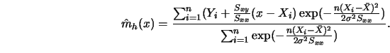
A ![]() analogue of the regressogram has also been proposed. Instead of
averaging the response variables in bins of fixed width, the statistically equivalent block regressogram is constructed by averaging
always over
analogue of the regressogram has also been proposed. Instead of
averaging the response variables in bins of fixed width, the statistically equivalent block regressogram is constructed by averaging
always over ![]() neighbors. The result is again a step function but now with
different lengths of the windows over which averaging is performed. Bosq and
Lecoutre (1987) consider consistency and rates of convergence of this
estimator.
neighbors. The result is again a step function but now with
different lengths of the windows over which averaging is performed. Bosq and
Lecoutre (1987) consider consistency and rates of convergence of this
estimator.
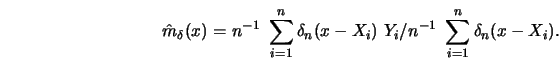
The idea of convolution smoothing was proposed by Clark (1977) and has
strong relations to kernel smoothing (see Section 3.1).
The CS-estimator (CS for convolution-smoothing) is defined as

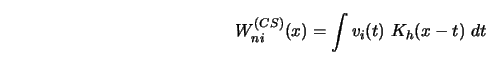
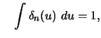
A delta function sequence (DFS) is a sequence of smooth weighting
functions
![]() , approximating the Dirac
, approximating the Dirac
![]() -function for large
-function for large ![]() . These DFSs
were used by Johnston (1979)
in forming the following type of regression estimator,
. These DFSs
were used by Johnston (1979)
in forming the following type of regression estimator,
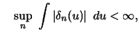
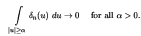
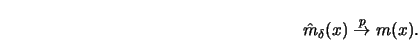
Under these general conditions on ![]() and continuity
assumptions on
and continuity
assumptions on ![]() and
and ![]() it can be shown that
it can be shown that
Suppose that the aim of approximation is the conditional median curve
med![]() rather than the conditional mean curve.
A sequence of ``local medians" of the response variables defines the
median smoother.
This estimator and related robust smoothers are
considered more theoretically in
Chapter 6, but it makes sense to already present it here since
median smoothing played a dominant role in the
historical evolution of smoothing techniques.
More formally, it is defined as
rather than the conditional mean curve.
A sequence of ``local medians" of the response variables defines the
median smoother.
This estimator and related robust smoothers are
considered more theoretically in
Chapter 6, but it makes sense to already present it here since
median smoothing played a dominant role in the
historical evolution of smoothing techniques.
More formally, it is defined as
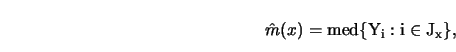

It has obvious similarities to the ![]() -
-![]() estimate (3.4.18)
but differs in at least two aspects: Median smoothing is highly resistant
to outliers and it is able to model unexpected discontinuities in
the regression curve med
estimate (3.4.18)
but differs in at least two aspects: Median smoothing is highly resistant
to outliers and it is able to model unexpected discontinuities in
the regression curve med![]() .
A comparison of both smoothing
techniques is given in Figure 3.16, which shows the motorcycle data
set (Table 1 in Appendix 2)
with a median smooth and a
.
A comparison of both smoothing
techniques is given in Figure 3.16, which shows the motorcycle data
set (Table 1 in Appendix 2)
with a median smooth and a ![]() -
-![]() smooth.
smooth.
![\includegraphics[scale=0.7]{ANRmotcompare.ps}](anrhtmlimg730.gif)
|
Note that the robustness aspect of median smoothing becomes visible here.
The median smooth is not influenced by a group of possible
outliers near ![]() and it is a little bit closer to the
main body of the data in the two ``peak regions"
and it is a little bit closer to the
main body of the data in the two ``peak regions" ![]() .
A slight
disadvantage is that by its nature, the median smooth is a rough
function.
.
A slight
disadvantage is that by its nature, the median smooth is a rough
function.
Median smoothing seems to require more
computing time than the ![]() -
-![]() estimate (due to sorting operations).
The simplest algorithm for running medians would sort in each window.
This would result in
estimate (due to sorting operations).
The simplest algorithm for running medians would sort in each window.
This would result in
![]() operations using a fast sorting routine.
Using the fast median algorithm by Bent and John (1985) this complexity
could be reduced to
operations using a fast sorting routine.
Using the fast median algorithm by Bent and John (1985) this complexity
could be reduced to ![]() operations. Härdle and Steiger (1988)
have shown that by maintaining a double heap structure as the window moves
over the span of the
operations. Härdle and Steiger (1988)
have shown that by maintaining a double heap structure as the window moves
over the span of the ![]() -variables, this complexity can be reduced to
-variables, this complexity can be reduced to
![]() operations. Thus running medians are only by a factor
of
operations. Thus running medians are only by a factor
of ![]() slower than
slower than ![]() -
-![]() smoothers.
smoothers.
A useful assumption for the mathematical analysis
of the nonparametric smoothing
method is the continuity of the underlying regression curve ![]() .
In some situations
a curve with steps, abruptly changing derivatives or even
cusps might be more appropriate than a smooth regression
function. McDonald and Owen (1986) give several examples:
These include Sweazy's kinked demand curve (Lipsey, Sparks and Steiner
1976) in microeconomics and daily readings of the sea surface
temperature. Figure 3.17 shows a
sawtooth function together with a kernel estimator.
.
In some situations
a curve with steps, abruptly changing derivatives or even
cusps might be more appropriate than a smooth regression
function. McDonald and Owen (1986) give several examples:
These include Sweazy's kinked demand curve (Lipsey, Sparks and Steiner
1976) in microeconomics and daily readings of the sea surface
temperature. Figure 3.17 shows a
sawtooth function together with a kernel estimator.
![\includegraphics[scale=0.7]{ANRsawtooth.ps}](anrhtmlimg737.gif)
|
The kernel estimation curve is
qualitatively smooth but by construction must blur the
discontinuity. McDonald and Owen (1986) point out that smoothing by
running medians has no trouble finding the discontinuity, but appears to
be very rough. They proposed, therefore, the split linear smoother.
Suppose that the ![]() -data are ordered, that is,
-data are ordered, that is,
![]() . The
split linear smoother begins by obtaining at
. The
split linear smoother begins by obtaining at ![]() a family of linear
fits corresponding to a family of windows. These windows are an ensemble
of neighborhoods of
a family of linear
fits corresponding to a family of windows. These windows are an ensemble
of neighborhoods of ![]() with different spans centered at
with different spans centered at ![]() or
having
or
having ![]() as their left boundary or right boundary. The split linear
smoother at point
as their left boundary or right boundary. The split linear
smoother at point ![]() is then obtained as a weighted average of the
linear fits there.
These weights depend on a measure of quality of the corresponding linear
fits. In Figure 3.18 the sawtooth data are presented together
with the split linear fit. This smoother
found the discontinuous sawtooth curve and is smooth elsewhere.
Theoretical aspects (confidence bands, convergence
to
is then obtained as a weighted average of the
linear fits there.
These weights depend on a measure of quality of the corresponding linear
fits. In Figure 3.18 the sawtooth data are presented together
with the split linear fit. This smoother
found the discontinuous sawtooth curve and is smooth elsewhere.
Theoretical aspects (confidence bands, convergence
to ![]() ) are described in Marhoul and Owen (1984).
) are described in Marhoul and Owen (1984).
![\includegraphics[scale=0.15]{ANR3,18.ps}](anrhtmlimg739.gif)
|
Schmerling and Peil (1985) proposed to estimate the unknown joint
density ![]() of
of ![]() and then to estimate
and then to estimate ![]() by the standard formula.
In particular, they proposed to use the mixture
by the standard formula.
In particular, they proposed to use the mixture
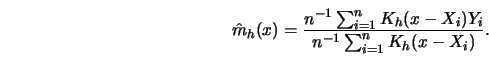
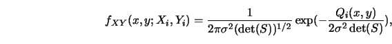
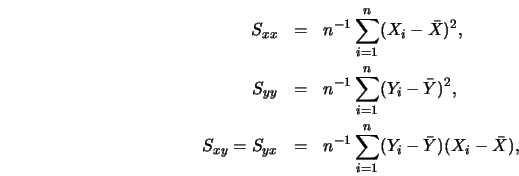

Figure 3.19 gives an impression of how this empirical regression curve works with real data. For more details I refer to Schmerling and Peil (1985).
![\includegraphics[scale=0.2]{ANR3,19.ps}](anrhtmlimg750.gif)
|
Exercises
3.10.1Vary the ``origin" of the regressogram, that is, define the bins
over which to average the response variable as

3.10.2Average the ![]() regressograms as defined in Exercise
3.10.5
Do you see any connection with the kernel technique?
[Hint: In Section 3.1 we called this Weighted Averaging over Rounded
Points the WARPing technique.]
regressograms as defined in Exercise
3.10.5
Do you see any connection with the kernel technique?
[Hint: In Section 3.1 we called this Weighted Averaging over Rounded
Points the WARPing technique.]
3.10.3Find a correspondence between the conditions (3.10.40) and the assumptions needed for the kernel consistency Proposition 3.1.1
Schmerling and Peil also considered more general polynomial fits than there introduced in Section 3.1. These local polynomial fits can be obtained by approximating polynomials of higher order or by using other kernels than the uniform kernel in (3.1.13); see also Katkovnik (1979, 1983, 1985) and Lejeune (1985).
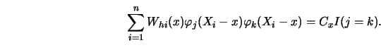
Suppose that ![]() is to be approximated by a polynomial
is to be approximated by a polynomial
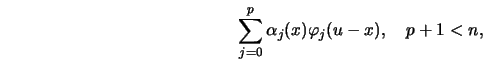
![\begin{displaymath}\sum_{i=1}^nW_{hi}(x)\ \left[ Y_i-\sum_{j=0}^p \alpha_j(x) \varphi_j
(X_i-x)\right]^2 {\buildrel ! \over =}\min \end{displaymath}](anrhtmlimg756.gif)
![\begin{displaymath}2 \sum_{i=1}^n W_{hi}(x)\ \left[ Y_i-\sum_{j=0}^p\alpha_j (x)\varphi_j
(X_i-x)\right] \varphi_k(X_i-x)=0, \ h=1,\ldots ,n. \end{displaymath}](anrhtmlimg758.gif)
![\begin{displaymath}\hat{\alpha}_j(x)= {\sum^n_{i=1} [W_{hi}(x) \varphi_j(X_i-x)]...
...um^n_{i=1} W_{hi}(x) \varphi^2_j (X_i-x)} ,\quad j=0,\ldots,p, \end{displaymath}](anrhtmlimg763.gif)
![\begin{displaymath}W^*_{hi}(x)= \sum^p_{j=0} \left[ {W_{hi}(x) \varphi_j (X_i-x)...
...m^n_{k=1} W_{hk}(x) \varphi^2_j (X_k-x) } \right] \varphi_j(0).\end{displaymath}](anrhtmlimg765.gif)