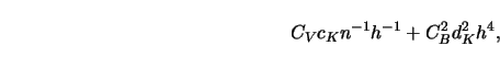
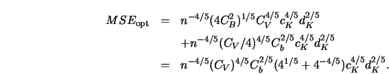
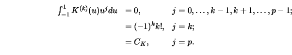
In Section 3.1 we have seen that the MSE of
![]() can be written as
can be written as
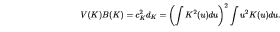
![\begin{displaymath}V(K)B(K)=\left[\int_{-1}^1 (K^{(k)}(u)^2 d u\right]^{p-k} \left \vert \int_{-1}^1
K^{(k)}(u)u^p d u \right \vert^{2 k+1}.\end{displaymath}](anrhtmlimg1318.gif)
To answer this question note first that we have to standardize the kernel
somehow since this functional of ![]() is invariant under scale transformations
is invariant under scale transformations
Gasser, Müller and Mammitzsch (1985) used variational methods to minimize
![]() with respect to
with respect to ![]() . The answers are polynomials of degree
. The answers are polynomials of degree ![]() .
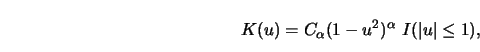
Some of these ``optimal'' kernels are presented in Table 4.1.
.
Some of these ``optimal'' kernels are presented in Table 4.1.
| kernel |
|||
| 0 | 2 |
|
|
| 0 | 4 |
|
|
| 1 | 3 |
|
|
| 1 | 5 |
|
|
| 2 | 4 |
|
|
| 2 | 6 |
|
|
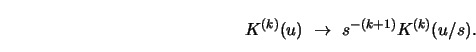
It is said that a kernel is of order ![]() if it satisfies the
following moment conditions:
if it satisfies the
following moment conditions:
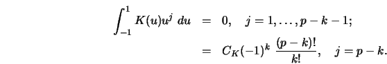
The optimal kernels given in Table 4.1 are of order ![]() . Another
important issue can be seen from Table 4.1 : Derivatives of ``optimal''
kernels do not yield ``optimal'' kernels for estimation of derivatives, for
example, the kernel for
. Another
important issue can be seen from Table 4.1 : Derivatives of ``optimal''
kernels do not yield ``optimal'' kernels for estimation of derivatives, for
example, the kernel for ![]() is not the derivative of the one with
is not the derivative of the one with
![]() . But note that the derivative of the latter kernel satisfies
4.5.28 with
. But note that the derivative of the latter kernel satisfies
4.5.28 with ![]() .
.
Figure 4.13 depicts two optimal kernels for ![]() and
and ![]() .
.
![\includegraphics[scale=0.7]{ANRoptker1.ps}](anrhtmlimg1337.gif)
|
Note that the kernel with ![]() has negative side lobes. The Epanechnikov
kernel is ``optimal'' for estimating
has negative side lobes. The Epanechnikov
kernel is ``optimal'' for estimating ![]() when
when ![]() . The kernel functions
estimating the first derivative must be odd functions by construction. A plot
of two kernels for estimating the first derivative of
. The kernel functions
estimating the first derivative must be odd functions by construction. A plot
of two kernels for estimating the first derivative of ![]() is given in Figure
4.14. The kernels for estimating second derivatives are even functions, as
can be seen from Figure 4.15. A negative effect of using higher order kernels
is that by construction they have negative side lobes. So a kernel smooth
(computed with a higher order kernel) can be partly negative even though it is
computed from purely positive response variables. Such an effect is
particularly undesirable in demand theory, where kernel smooths are used to
approximate statistical Engel curves; see Bierens (1987).
is given in Figure
4.14. The kernels for estimating second derivatives are even functions, as
can be seen from Figure 4.15. A negative effect of using higher order kernels
is that by construction they have negative side lobes. So a kernel smooth
(computed with a higher order kernel) can be partly negative even though it is
computed from purely positive response variables. Such an effect is
particularly undesirable in demand theory, where kernel smooths are used to
approximate statistical Engel curves; see Bierens (1987).
![\includegraphics[scale=0.7]{ANRoptker2.ps}](anrhtmlimg1341.gif)
|
![\includegraphics[scale=0.7]{ANRoptker3.ps}](anrhtmlimg1344.gif)
|
A natural question to ask is, how ``suboptimal'' are nonoptimal kernels, that
is, by how much the expression ![]() is increased for nonoptimal kernels?
Table 4.2 lists some commonly used kernels (for
is increased for nonoptimal kernels?
Table 4.2 lists some commonly used kernels (for ![]() ) and Figure
4.16
gives a graphical impression of these kernel. Their deficiencies with respect
to the Epanechnikov kernel are defined as
) and Figure
4.16
gives a graphical impression of these kernel. Their deficiencies with respect
to the Epanechnikov kernel are defined as
![\begin{displaymath}D(K_{\textrm{opt}}, K)=[V(K_{\textrm{opt}})B(K_{\textrm{opt}})]^{-1} [V(K)B(K)].\end{displaymath}](anrhtmlimg1346.gif)
| Kernel |
|
|
| Epanechnikov |
|
1 |
| Quartic |
|
1.005 |
| Triangular |
|
1.011 |
| Gauss |
|
1.041 |
| Uniform |
|
1.060 |
A picture of these kernels is given in Figure 4.16. The kernels really look different, but Table 4.2 tells us that their MISE behavior is almost the same.
![\includegraphics[scale=0.7]{ANRposkernels.ps}](anrhtmlimg1354.gif)
|
The bottom line of Table 4.2 is that the choice between the various kernels on the basis of the mean squared error is not very important. If one misses the optimal bandwidth minimizing MISE (or some other measure of accuracy) by 10 percent there is a more drastic effect on the precision of the smoother than if one selects one of the ``suboptimal'' kernels. It is therefore perfectly legitimate to select a kernel function on the basis of other considerations, such as the computational efficiency (Silverman 1982; Härdle, 1987a).
Exercises
4.5.1 Verify the ``small effect of choosing the wrong kernel'' by a
Monte Carlo study. Choose

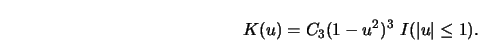
4.5.2 Compute ![]() for the triweight kernel
for the triweight kernel
4.5.3 Prove that ![]() as defined in
4.5.28 is invariant under
the scale transformations 4.5.29.
as defined in
4.5.28 is invariant under
the scale transformations 4.5.29.
4.5.4 A colleague has done the Monte Carlo study from Exercise
4.5 in
the field of density smoothing. His setting was
| estimated | ||
| Kernel | MSE | interval |
| Epanechnikov | 0.002214 | |
| Quartic | 0.002227 | |
| Triangular | 0.002244 | |
| Gauss | 0.002310 | |
| Uniform | 0.002391 |
Do these numbers correspond to the values
![]() from Table
4.2?
from Table
4.2?
I give a sketch of a proof for the optimality of the Epanechnikov kernel.
First, we have to standardize the kernel since ![]() is invariant under
scale transformations. For reasons that become clear in Section
5.4 I use the
standardization
is invariant under
scale transformations. For reasons that become clear in Section
5.4 I use the
standardization ![]() . The task for optimizing
. The task for optimizing ![]() is then to
minimize
is then to
minimize
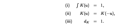
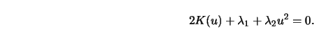
If ![]() denotes a small variation for an extremum subject to the
constraints (i)-(iii), the variation of
denotes a small variation for an extremum subject to the
constraints (i)-(iii), the variation of
![\begin{displaymath}\int K^2(u) d u+\lambda_1 \left[\int K(u) d u-1\right]+\lambda_2 \left[\int
u^2 K(u) d u- 1\right]\end{displaymath}](anrhtmlimg1369.gif)
![\begin{displaymath}2 \int K(u)\Delta K(u) d u+\lambda_1 \left[\int \Delta K(u) d u\right
]+\lambda_2 \left[\int \Delta K(u) u^2\right]=0.\end{displaymath}](anrhtmlimg1370.gif)