Before we get to the details it might be a good idea to take a
look at the end product of the procedure.
If you look at Figure 2.6 you can see a ``histogram'' that
has been obtained
by averaging over eight histograms corresponding to different
origins (four of these eight histograms are plotted in
Figure 2.7).
Figure:
Averaged
shifted histogram for stock returns data; average of 8 histograms
with origins 0,  ,
,  ,
,  ,
,  ,
,  ,
,  ,
,
 ,
,  and binwidth
![\includegraphics[width=0.03\defepswidth]{quantlet.ps}](spmhtmlimg1.gif) SPMashstock
SPMashstock
|
|
The resulting averaged shifted histogram (ASH) is freed from the dependency of the origin and seems to
correspond to a smaller binwidth than the
histograms from which it was constructed. Even though the ASH
can in some sense (which will be made more precise below) be viewed
as having a smaller binwidth, you should be aware that it is not simply an ordinary histogram with a smaller binwidth (as you
can easily see by looking at Figure 2.7 where we graphed
an ordinary histogram with a comparable binwidth and origin  ).
).
Figure:
Ordinary
histogram for stock returns; binwidth 
SPMhiststock
|
|
Let us move on to the details. Consider a bin grid corresponding to
a histogram with origin and bins
 ,
,
 , i.e.
Let us generate  new bin grids by shifting each
  by
the amount
by
the amount  to the right
 |
(2.27) |
EXAMPLE 2.1
As an example take

:
Of course if we take

then we get the original bin grid,
i.e.

.

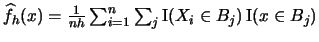
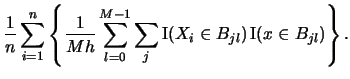
Now suppose we calculate a histogram for each of the  bin
grids.
Then we get different estimates for
bin
grids.
Then we get different estimates for  at each
 |
(2.28) |
The ASH is obtained by averaging over these estimates
As
 , the ASH is not dependent on the origin
anymore and converts from a step function into a continuous
function. This asymptotic behavior can be directly achieved
by a different technique: kernel density estimation, studied
in detail in the following Section 3.
, the ASH is not dependent on the origin
anymore and converts from a step function into a continuous
function. This asymptotic behavior can be directly achieved
by a different technique: kernel density estimation, studied
in detail in the following Section 3.
Additional material on the histogram can be found in
Scott (1992) who in specifically covers rules for the optimal
number of bins, goodness-of-fit criteria and
multidimensional histograms.
A related density estimator is the frequency polygon which is
constructed by interpolating the histogram values
 .
This yields a piecewise linear but now continuous estimate of the
density function. For details and asymptotic properties see
Scott (1992, Chapter 4).
.
This yields a piecewise linear but now continuous estimate of the
density function. For details and asymptotic properties see
Scott (1992, Chapter 4).
The idea of averaged shifted histograms can be used to motivate
the kernel density estimators introduced in the following
Chapter 3. For this application we refer to
Härdle (1991) and Härdle & Scott (1992).
EXERCISE 2.5
Prove that for every density function
, which is a step function,
i.e.
the histogram

defined on the bins

is the
maximum likelihood estimate.
EXERCISE 2.6
Simulate a sample of standard normal distributed random variables
and compute an optimal histogram corresponding to the optimal
binwidth

in this case.
EXERCISE 2.7
Consider
![$ f(x)=2x\cdotp\Ind(x\in[0,1])$](spmhtmlimg549.gif)
and histograms using binwidths

for

starting at

.
Calculate
and the optimal binwidth
.
(Hint: The solution is
EXERCISE 2.8
Recall that for

to be a consistent estimator of

it has to be true that
for any

holds
, i.e. it has to be true that
converges in
probability. Why is it sufficient to show that
converges to 0?
EXERCISE 2.10
Explain in detail why for the standard normal pdf

we obtain
EXERCISE 2.11
The optimal binwidth

that minimizes

for

is
. How does this
rule of thumb change for

and

?
EXERCISE 2.12
How would the formula for the histogram change
if we based it on intervals of the form
instead
of
?
EXERCISE 2.13
Show that the histogram

is a maximum likelihood estimator of
for an arbitrary
discrete distribution, supported by {0,1,...}, if one considers

and
,

.
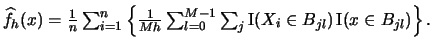
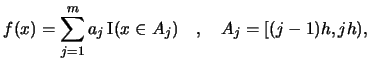
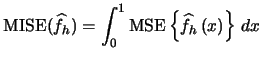
Summary

- A histogram with binwidth
 and origin
  is defined
by
is defined
by
 where
where
 and
.
and
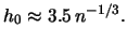
.
- The bias of a histogram is
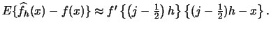
- The variance of a histogram is
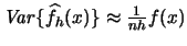 .
.
- The asymptotic
 is given by
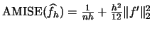 .
.
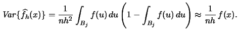
- The optimal binwidth that minimizes is
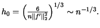
- The optimal binwidth
that minimizes for is
- The averaged shifted histogram (ASH) is given by
 The ASH is less dependent on the origin as the ordinary histogram.
![\includegraphics[width=1.2\defpicwidth]{SPMashstock.ps}](spmhtmlimg522.gif)
![\includegraphics[width=1.2\defpicwidth]{SPMhiststock.ps}](spmhtmlimg524.gif)
![$\displaystyle f(x)=\frac{2}{3}\left[ \left(\frac{x}{2} +1\right)
\Ind\{x\in[-2,0)\} + (1-x)\Ind\{x\in[0,1)\}\right]$](spmhtmlimg559.gif)