Stock prices are stochastic processes in discrete time which
take only discrete values due to the limited measurement
scale. Nevertheless, stochastic processes in continuous time
are used as models since they are analytically easier to handle
than discrete models, e.g. the binomial or trinomial process.
However, the latter are more intuitive and prove to be very useful
in simulations.
Two features of the general Wiener process
 make it an unsuitable model for stock prices. First, it
allows for negative stock prices, and second the local variability
is higher for high stock prices. Hence, stock prices
make it an unsuitable model for stock prices. First, it
allows for negative stock prices, and second the local variability
is higher for high stock prices. Hence, stock prices  are
modeled by means of the more general Itô-process:
are
modeled by means of the more general Itô-process:
This model does depend on the unknown functions
 and
and
 A useful and simpler variant utilizing only two
unknown real model parameters
A useful and simpler variant utilizing only two
unknown real model parameters  and
and  can be justified
by the following reflection: The percentage return on the invested
capital should on average not depend on the stock price at which
the investment is done, and of course, should not depend on the
currency unit (EUR, USD, ...) in which the stock price
is quoted. Furthermore, the average return should be proportional
to the investment horizon, as it is the case for other investment
instruments. Putting things together, we request:
Since
can be justified
by the following reflection: The percentage return on the invested
capital should on average not depend on the stock price at which
the investment is done, and of course, should not depend on the
currency unit (EUR, USD, ...) in which the stock price
is quoted. Furthermore, the average return should be proportional
to the investment horizon, as it is the case for other investment
instruments. Putting things together, we request:
Since
![$ \mathop{\text{\rm\sf E}}[dW_t] = 0$](sfehtmlimg764.gif) this condition is satisfied if
for given
this condition is satisfied if
for given  Additionally,
takes into consideration that the absolute size of the stock price
fluctuation is proportional to the currency unit in which the
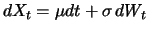
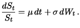
stock price is quoted. In summary, we model the stock price
as a solution of the stochastic differential equation
where is the expected return on the stock, and
the volatility. Such a process is called geometric Brownian motion because
By applying Itôs lemma, which we introduce in Section
5.5, it can be shown that for a suitable Wiener
process
Additionally,
takes into consideration that the absolute size of the stock price
fluctuation is proportional to the currency unit in which the
stock price is quoted. In summary, we model the stock price
as a solution of the stochastic differential equation
where is the expected return on the stock, and
the volatility. Such a process is called geometric Brownian motion because
By applying Itôs lemma, which we introduce in Section
5.5, it can be shown that for a suitable Wiener
process
 it holds

bzw.
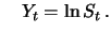
Since  is normally distributed, is lognormally
distributed. As random walks can be used to approximate the
general Wiener process, geometric random walks can be used to
approximate geometric Brownian motion and thus this simple model
for the stock price.
is normally distributed, is lognormally
distributed. As random walks can be used to approximate the
general Wiener process, geometric random walks can be used to
approximate geometric Brownian motion and thus this simple model
for the stock price.
Fig.:
Density comparison of lognormally and normally
distributed random variables.
 SFELogNormal.xpl
|
|
![$\displaystyle \frac{\mathop{\text{\rm\sf E}}[dS_t]}{S_t} \, = \, \frac{\mathop{\text{\rm\sf E}}[S_{t+dt} - S_t]}{S_t} \, = \,
\mu \cdot dt \, . $](sfehtmlimg763.gif)
![\includegraphics[width=1\defpicwidth]{distrib.ps}](sfehtmlimg772.gif)