12.4 Partial Autocorrelation

For a given stochastic process one is often interested in the connection between two random variables of a process at different points in time. One way to measure a linear relationship is with the ACF, i.e., the correlation between these two variables. Another way to measure the connection between $X_{t}$ and $X_{t+\tau}$ is to filter out of $X_{t}$ and $X_{t+\tau}$ the linear influence of the random variables that lie in between, $X_{t+1},\ldots,X_{t+\tau-1},$ and then calculate the correlation of the transformed random variables. This is called the partial autocorrelation.

Definition 12.3 (Partial autocorrelation)  
The partial autocorrelation of $k-$th order is defined as

$$\phi_{kk} = \mathop{\text{\rm Corr}}(X_t-{\cal P}(X_t\mid X_{t+1},\ldots,X_{t+k-1}),$$

$$\qquad X_{t+k}-{\cal P}(X_{t+k}\mid X_{t+1},\ldots,X_{t+k-1}))$$ (12.17)

where ${\cal P}(W\mid Z)$ is the best linear projection of $W$ on $Z$, i.e., ${\cal P}(W\mid Z)=\Sigma_{WZ}\Sigma_{ZZ}^{-1}Z$ with $\Sigma_{ZZ}=\mathop{\text{\rm Var}}(Z)$ as the covariance matrix of the regressors and $\Sigma_{WZ}=\mathop{\text{\rm Cov}}(W,Z)$ as the matrix of covariances between $W$ and $Z$.

The `best linear projection' is understood in the sense of minimizing the mean squared error.

An equivalent definition is the solution to the system of equations

$$P_k \phi_k = \rho_{(k)}$$

with

$$P_k = \left( \begin{array}{*{3}{c}cc} 1 & \rho_1 & \cdots & ... ...s \\ \rho_{k-1} & \rho_{k-2} & \cdots & 1 \end{array}\right )$$

$\phi_k = (\phi_{k1}, \ldots, \phi_{kk})^\top$ and $\rho_{(k)} = (\rho_{1}, \ldots, \rho_{k})^\top$. These are the Yule-Walker equations for an AR($k$) process. The last coefficient, $\phi_{kk}$, is the partial autocorrelation of order $k$, as defined above. Since only this coefficient is of interest in this context, the system of equations can be solved for $\phi_{kk}$ using the Cramer-Rule. We get

$$\phi_{kk} = \frac{\vert P_k^*\vert}{\vert P_k\vert}$$

where $P_k^*$ is equal to the matrix $P_k$, in which the $k-$th column is replaced with $\rho_{(k)}$. Here $\vert.\vert$ indicates the determinant. Since this can be applied for various orders $k$, in the end we obtain a partial autocorrelation function (PACF). The PACF can be graphically displayed for a given stochastic process, similar to the ACF as a function of order $k$. This is called the partial autocorrelogram.

From the definition of PACF it immediately follows that there is no difference between PACF and ACF of order 1:

$$\phi_{11} = \rho_1.$$

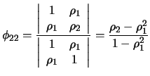
For order 2 we have

$$\phi_{22} = \frac{ \left\vert \begin{array}{cc} 1 & \rho_1 \\ \rh... ...\rho_1 & 1 \\ \end{array} \right \vert } = \frac{\rho_2 - \rho_1^2}{1-\rho_1^2}$$ (12.18)

Example 12.3 (AR(1))  
The AR(1) process $X_t = \alpha X_{t-1} + \varepsilon_t$ has the ACF $\rho_{\tau}=\alpha^{\tau}$. For the PACF we have $\phi_{11}=\rho_1=\alpha$ and

$$\phi_{22}=\frac{\rho_2-\rho_1^2}{1-\rho_1^2}=\frac{\alpha^2-\alpha^2}{1-\alpha^2}=0,$$

and $\phi_{kk}=0$ for all $k>1$. This is plausible since the last coefficient of an AR($k$) model for this process is zero for all $k>1$. For $k=2$ we illustrate the equivalence with Definition 11.3: From $X_t = \alpha X_{t-1} + \varepsilon_t$ we directly obtain ${\cal P}(X_{t+2}\vert X_{t+1})=\alpha X_{t+1}$ with

$$\alpha=\frac{\mathop{\text{\rm Cov}}(X_{t+2},X_{t+1})}{\mathop{\text{\rm Var}}(X_{t+1})}.$$

From the 'backward regression' $X_t=\alpha^{\prime}X_{t+1}+\eta_t$ with white noise $\eta_t$ it further follows that ${\cal P}(X_{t}\vert X_{t+1})=\alpha^{\prime} X_{t+1}$ with

$$\alpha^{\prime}=\frac{\mathop{\text{\rm Cov}}(X_{t},X_{t+1})}{\mathop{\text{\rm Var}}(X_{t+1})}.$$

For $\vert\alpha\vert < 1$ the process is covariance-stationary and it holds that
$\mathop{\text{\rm Cov}}(X_{t+2},X_{t+1})=\mathop{\text{\rm Cov}}(X_{t},X_{t+1})=\gamma_1$ and $\alpha=\alpha^{\prime}=\rho_1$. We obtain

$$\mathop{\text{\rm Cov}}\{X_t-{\cal P}(X_t\vert X_{t+1}),X_{t+2}-{\cal P}(X_{t+2}\vert X_{t+1})\}$$

$$= \mathop{\text{\rm Cov}}(X_t-\rho_1 X_{t+1},X_{t+2}-\rho_1 X_{t+1})$$

$$= \mathop{\text{\rm\sf E}}[(X_t-\rho_1 X_{t+1})(X_{t+2}-\rho_1 X_{t+1})]$$

$$= \gamma_2 - 2\rho_1 \gamma_1 + \rho_1^2 \gamma_0$$

and

$$\mathop{\text{\rm Var}}\{X_{t+2}-{\cal P}(X_{t+2}\vert X_{t+1})\} = \mathop{\text{\rm\sf E}}[(X_{t+2}-\rho_1X_{t+1})^2]$$

$$= \gamma_0(1+\rho_1^2)-2\rho_1\gamma_1$$

$$= \mathop{\text{\rm\sf E}}[(X_{t}-\rho_1 X_{t+1})^2]$$

$$= \mathop{\text{\rm Var}}[X_{t}-{\cal P}(X_{t}\vert X_{t+1})].$$

With this we get for the partial autocorrelation of 2nd order

$$\phi_{22} = \mathop{\text{\rm Corr}}\{X_t-{\cal P}(X_t\vert X_{t+1}),X_{t+2}-{\cal P}(X_{t+2}\vert X_{t+1})\}$$

$$= \frac{\mathop{\text{\rm Cov}}\{X_t-{\cal P}(X_t\vert X_{t+1}),X_{... ...X_{t+1})\}} \sqrt{\mathop{\text{\rm Var}}(X_{t}-{\cal P}(X_{t}\vert X_{t+1}))}}$$

$$= \frac{\gamma_2-2\rho_1\gamma_1 + \rho_1^2\gamma_0}{\gamma_0(1+\rho_1^2)-2\gamma_1\rho_1}$$

$$= \frac{\rho_2 - \rho_1^2}{1-\rho_1^2}$$

which corresponds to the results in (11.18). For the AR(1) process it holds that $\rho_2=\rho_1^2$ and thus $\phi_{22}=0$.

It holds in general for AR($p$) processes that $\phi_{kk}=0$ for all $k>p$. In Figure 11.5 the PACF of an AR(2) process is displayed using the parameters as in Figure 11.4.

Fig.: PACF of an AR(2) process with $(\alpha_1=0.5,\alpha_2=0.4)$ (top left), $(\alpha_1=0.9,\alpha_2=-0.4)$ (top right), $(\alpha_1=-0.4,\alpha_2=0.5)$ (bottom left) and $(\alpha_1=-0.5,\alpha_2=-0.9)$ (bottom right). SFEpacfar2.xpl

Example 12.4 (MA(1))  
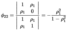
For a MA(1) process $X_t = \beta \varepsilon_{t-1}+\varepsilon_t$ with $\mathop{\text{\rm Var}}(\varepsilon_t)=\sigma^2$ it holds that $\gamma_0=\sigma^2(1+\beta^2)$, $\rho_1 = \beta/(1+\beta^2)$ and $\rho_k=0$ for all $k>1$. For the partial autocorrelations we obtain $\phi_{11}=\rho_1$ and

$$\phi_{22} = \frac{ \left\vert \begin{array}{cc} 1 & \rho_1 \\ \rh... ...o_1 \\ \rho_1 & 1 \\ \end{array} \right \vert } = - \frac{\rho_1^2}{1-\rho_1^2}$$ (12.19)

For a MA(1) process it strictly holds that $\phi_{22}<0$. If one were to continue the calculation with $k>2$, one could determine that the partial autocorrelations will not reach zero.

Figure 11.6 shows the PACF of a MA(2) process. In general for a MA($q$) process it holds that the PACF does not decay, in contrast to the autoregressive process. Compare the PACF to the ACF in Figure 11.2. This is thus a possible criterium for the specification of a linear model.

Fig.: PACF of a MA(2) process with $(\beta_1=0.5,\beta_2=0.4)$ (top left), $(\beta_1=0.5,\beta_2=-0.4)$ (top right), $(\beta_1=-0.5,\beta_2=0.4)$ (bottom left) and $(\beta_1=-0.5,\beta_2=-0.4)$ (bottom right). SFEpacfma2.xpl