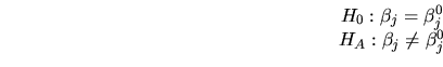
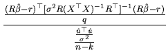
The previous sections have developed, through point and interval estimation, a method to infer a population value from a sample. Hypothesis testing constitutes another method of inference which consists of formulating some assumptions about the probability distribution of the population from which the sample was extracted, and then trying to verify these assumptions for them to be considered adequate. In this sense, hypothesis testing can refer to the systematic component of the model as well as its random component. Some of these procedures will be studied in the following chapter of this book, whilst in this section we only focus on linear hypotheses about the coefficients and the parameter of dispersion of the MLRM.
In order to present how to compute hypothesis testing about the
coefficients, we begin by considering the general statistic which
allows us to test any linear restrictions on ![]() . Afterwards,
we will apply this method to particular cases of interest, such as
the hypotheses about the value of a
. Afterwards,
we will apply this method to particular cases of interest, such as
the hypotheses about the value of a ![]() coefficient, or
about all the coefficients excepting the intercept.
coefficient, or
about all the coefficients excepting the intercept.
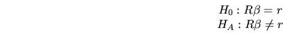
In order to test any linear hypothesis about the coefficient, the problem is formulated as follows:
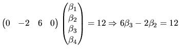
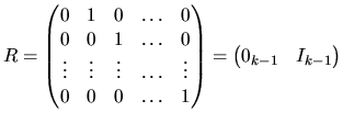
The matrix ![]() and the vector
and the vector ![]() can be considered as artificial
instruments which allow us to express any linear restrictions in
matrix form. To illustrate the role of these instruments, consider
an MLRM with 4 coefficients. For example, if we want to test
can be considered as artificial
instruments which allow us to express any linear restrictions in
matrix form. To illustrate the role of these instruments, consider
an MLRM with 4 coefficients. For example, if we want to test

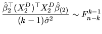
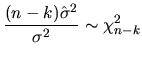
Expression (2.138) includes the unknown parameter
![]() , so in order to obtain a value for the statistic, we
have to use the independence between the quadratic form given in
(2.138), and the distribution (2.125)
is (see Hayashi (2000)), in such a way that:
, so in order to obtain a value for the statistic, we
have to use the independence between the quadratic form given in
(2.138), and the distribution (2.125)
is (see Hayashi (2000)), in such a way that:
A way of solving this question consists of employing the so-called
p-value provided by a sample in a specific test. It can be defined
as the lowest significance level which allows us to reject
![]() , with the available sample:
, with the available sample:
It we use the p-value, the decision rule is modified in stages ![]() and
and ![]() as follows:
as follows: ![]() to calculate the p-value, and
to calculate the p-value, and ![]() if
if
![]() ,
, ![]() is accepted. Otherwise, it is
rejected.
is accepted. Otherwise, it is
rejected.
Econometric softwar does not usually contain the general
F-statistic, except for certain particular cases which we will
discuss later. So, we must obtain it step by step, and it will not
always be easy, because we have to calculate the inverses and
products of matrices. Fortunately, there is a convenient
alternative way involving two different residual sum of squares
(![]() ): that obtained from the estimation of the MLRM, now
denoted
): that obtained from the estimation of the MLRM, now
denoted ![]() (unrestricted residual sum of squares), and that
called restricted residual sum of squares, denoted
(unrestricted residual sum of squares), and that
called restricted residual sum of squares, denoted ![]() . The
latter is expressed as:
. The
latter is expressed as:

If we use (2.140) to test a linear hypothesis about
![]() , we only need to obtain the
, we only need to obtain the ![]() corresponding to both
the estimation of the specified MLRM, and the estimation once we
have substituted the linear restriction into the model. The
decision rule does not vary: if
corresponding to both
the estimation of the specified MLRM, and the estimation once we
have substituted the linear restriction into the model. The
decision rule does not vary: if ![]() is true,
is true, ![]() should
not be much different from
should
not be much different from ![]() , and consequently, small
values of the statistic provide evidence in favour of
, and consequently, small
values of the statistic provide evidence in favour of ![]() .
.
Having established the general F statistic, we now analyze the most useful particular cases.
To obtain (2.142) we must note that, under ![]() , the
, the
![]() matrix becomes a row vector with zero value for each element,
except for the
matrix becomes a row vector with zero value for each element,
except for the ![]() element which has 1 value, and
element which has 1 value, and
![]() . Thus, the term
. Thus, the term
![]() becomes
becomes
![]() . Element
. Element
![]() becomes
becomes
![]() .
.
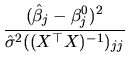
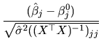
Moreover, we know that the squared root of the F random variable expressed in (2.142) follows a t-student whose degrees of freedom are those of the denominator of the F distribution, that is to say,
It must be noted that, given the form of ![]() in
(2.141), (2.143) is a two-tailed test, so
once we have calculated the statistic value
in
(2.141), (2.143) is a two-tailed test, so
once we have calculated the statistic value ![]() ,
, ![]() is
rejected if
is
rejected if
![]() .
.
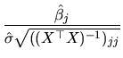
An interesting particular case of the t-statistic consists of
testing
![]() , which simplifies (2.143),
yielding:
, which simplifies (2.143),
yielding:
The statistic given in (2.143) is the same as
(2.122), which was derived in order to obtain the
interval estimation for a ![]() coefficient. This leads us
to conclude that there is an equivalence between creating a
confidence interval and carrying out a two-tailed test of the
hypothesis (2.141). In this sense, the confidence
interval can be considered as an alternative way of testing
(2.141). The decision rule will be: given a fixed
level of significance
coefficient. This leads us
to conclude that there is an equivalence between creating a
confidence interval and carrying out a two-tailed test of the
hypothesis (2.141). In this sense, the confidence
interval can be considered as an alternative way of testing
(2.141). The decision rule will be: given a fixed
level of significance ![]() and calculating a
and calculating a
![]() percent confidence interval, if the
percent confidence interval, if the ![]() value in
value in ![]() (
(
![]() ) belongs to the interval, we
accept the null hypothesis, at a level of significance
) belongs to the interval, we
accept the null hypothesis, at a level of significance ![]() .
Otherwise,
.
Otherwise, ![]() should be rejected. Obviously, this equivalence
holds if the significance level in the interval is the same as
that of the test.
should be rejected. Obviously, this equivalence
holds if the significance level in the interval is the same as
that of the test.
 |
(2.146) |
| (2.147) |
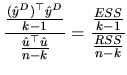
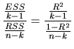
Nevertheless, the F statistic (2.148) has an
alternative form as a function of the explained sum of squares
![]() . To prove it, we begin by considering:
. To prove it, we begin by considering:
| (2.149) |
Furthermore, from the definition of ![]() given in (2.130)
we can deduce that:
given in (2.130)
we can deduce that:
We must note that the equivalence between (2.148) and (2.151) is only given when the MLRM has a constant term.
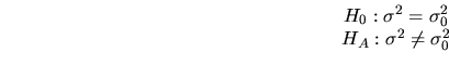
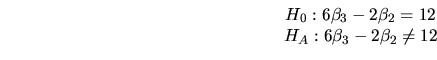
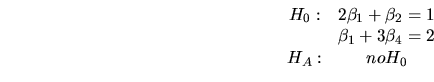
The earlier mentioned relationship between the confidence interval and hypothesis testing, allows us to derive the test of the following hypothesis easily:
Now, we present the quantlet
 linreg
in the
stats
quantlib which allows us to obtain the main measures of fit and
testing hypothesis that we have just described in both this
section and the previous section.
linreg
in the
stats
quantlib which allows us to obtain the main measures of fit and
testing hypothesis that we have just described in both this
section and the previous section.
|
For the example of the consumption function which we presented in previous sections, the quantlet XEGmlrm05.xpl obtains the statistical information
The column ![]() represents the squared sum of the regression
(ESS), the squared sum of the residuals (RSS) and the total
squared sum (TSS). The
represents the squared sum of the regression
(ESS), the squared sum of the residuals (RSS) and the total
squared sum (TSS). The ![]() column represents the means of
column represents the means of ![]() calculated by dividing
calculated by dividing ![]() by the corresponding degrees of
freedom(df). The F-test is the statistic to test
by the corresponding degrees of
freedom(df). The F-test is the statistic to test
![]() , which is followed by the
corresponding p-value. Afterwards, we have the measures of fit we
presented in the previous section, that is to say,
, which is followed by the
corresponding p-value. Afterwards, we have the measures of fit we
presented in the previous section, that is to say, ![]() ,
adjusted-
,
adjusted-![]() (
(
![]() ), and Standard Error (SER).
Moreover, multiple R represents the squared root of
), and Standard Error (SER).
Moreover, multiple R represents the squared root of ![]() .
.
Finally, the output presents the columns of the values of the
estimated coefficients (beta) and their corresponding standard
deviations (SE). It also presents the t-ratios (t-test) together
with their corresponding p-values. By observing the p-values, we
see that all the p-values are very low, so we reject
![]() , whatever the significance level (usually 1, 5
or 10 percent), which means that all the coefficients are
statistically significant. Moreover, the p-value of the F-tests
also allows us to conclude that we reject
, whatever the significance level (usually 1, 5
or 10 percent), which means that all the coefficients are
statistically significant. Moreover, the p-value of the F-tests
also allows us to conclude that we reject
![]() , or in other words, the overall
regression explains the
, or in other words, the overall
regression explains the ![]() variable. Finally, with this quntlet
it is also possible to illustrate the computation of the F
statistic to test the hypothesis
variable. Finally, with this quntlet
it is also possible to illustrate the computation of the F
statistic to test the hypothesis
![]() .
.
![$\displaystyle =\frac{(R\hat{\beta}-r)^{\top }[R(X^{\top }X)^{-1}R^{\top }]^{-1}(R\hat{\beta}-r)}{q\hat{\sigma}^{2}} \sim F^{q}_{n-k}$](xegbohtmlimg750.gif)