Regression smoothing investigates the association
between an explanatory variable ![]() and a response variable
and a response variable ![]() .
This section explains how to apply Nadaraya-Watson and local
polynomial kernel regression.
.
This section explains how to apply Nadaraya-Watson and local
polynomial kernel regression.
Nonparametric regression aims to estimate the functional
relation between ![]() and
and ![]() , i.e. the conditional expectation
, i.e. the conditional expectation
| (6.11) |
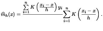
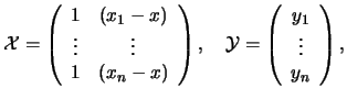
Suppose that we have independent observations
![]() . The Nadaraya-Watson estimator
is defined as
. The Nadaraya-Watson estimator
is defined as
The computational effort for calculating a Nadaraya-Watson or local polynomial regression is in the same order as for kernel density estimation (see Section 6.1.1). As in density estimation, all routines are offered in an exact and in a WARPing version:
| Functionality | Exact | WARPing |
| Nadaraya-Watson regression |  regxest
 |
regest |
| Nadaraya-Watson confidence intervals |
regxci |
regci |
| Nadaraya-Watson confidence bands |
regxcb |
regcb |
| Nadaraya-Watson bandwidth selection |
regxbwsel |
regbwsel |
| local polynomial regression |
lpregxest |
lpregest |
| local polynomial derivatives |
lpderxest |
lpderest |
The WARPing-based function
regest
offers the fastest way to
compute the
Nadaraya-Watson regression estimator for exploratory purposes.
We apply this routine
nicfoo
data, which contain observations
on household netincome in the first column and on food expenditures
in the second column. The following quantlet computes and plots
the regression curve together with the data:
  nicfoo=read("nicfoo")
  h=0.2*(max(nicfoo[,1])-min(nicfoo[,1]))
  mh=regest(nicfoo,h)
  mh=setmask(mh,"line","blue")
  xy=setmask(nicfoo,"cross","small")
  plot(xy,mh)
  setgopt(plotdisplay,1,1,"title","regression estimate")
regest
needs to be replaced by
regxest
,
if one is interested in the fitted values for all observations
  mh=regxest(nicfoo,0.2)
  res=nicfoo[,1] ~ (nicfoo[,2]-mh[,2])
  res=setmask(res,"cross")
  zline=(min(nicfoo[,1])|max(nicfoo[,1])) ~ (0|0)
  zline=setmask(zline,"line","red")
  plot(res,zline)
  setgopt(plotdisplay,1,1,"title","regression residuals")
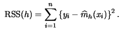
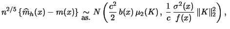
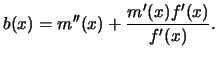
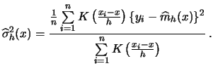
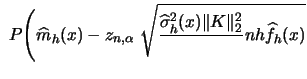
The resulting regression function is shown in Figure 6.8. Figure 6.9 shows the resulting residual plot. We observe that most of the nonlinear structure of the data is captured by the nonparametric regression function. However, the residual graph shows that the data are heteroskedastic, in the way that the residual variance increases with increasing netincome.
As in kernel density estimation, kernel regression involves
choosing the kernel function and the bandwidth parameter.
One observes the same phenomenon as in kernel density estimation
here: The difference between two kernel functions ![]() is almost
negligible when the bandwidths are appropriately rescaled.
To make the bandwidths for two different kernels
is almost
negligible when the bandwidths are appropriately rescaled.
To make the bandwidths for two different kernels ![]() comparable,
the same technique as described in Subsection 6.1.3
can be used.
comparable,
the same technique as described in Subsection 6.1.3
can be used.
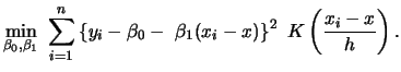
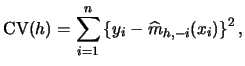
Consequently, we now concentrate on the problem of bandwidth selection. In the regression case, typically the averaged squared error
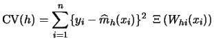 |
(6.14) |
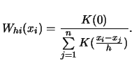
All the mentioned penalty functions
have the same asymptotic properties. In finite samples,
however, the functions differ in the relative weight
they give to variance and bias of
![]() .
Rice's
.
Rice's ![]() gives the most weight to variance reduction
while Shibata's model selector stresses bias reduction
the most.
gives the most weight to variance reduction
while Shibata's model selector stresses bias reduction
the most.
In
XploRe
, all penalizing functions can be applied via the
functions
regbwsel
and
regxbwsel
. As can
be seen from (6.13), criteria like
![]() need to
be evaluated at all observations. Thus, the function
regxbwsel
which uses exact computations is to
be preferred here.
regbwsel
uses the WARPing
approximation and may select bandwidths far from the
optimal, if the discretization binwidth
need to
be evaluated at all observations. Thus, the function
regxbwsel
which uses exact computations is to
be preferred here.
regbwsel
uses the WARPing
approximation and may select bandwidths far from the
optimal, if the discretization binwidth ![]() large.
Note that both
regbwsel
and
regxbwsel
may suffer from numerical problems if the studied bandwidths
are too small.
large.
Note that both
regbwsel
and
regxbwsel
may suffer from numerical problems if the studied bandwidths
are too small.
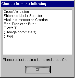
An example for calling
regxbwsel
gives the following
quantlet which uses the
nicfoo
data again:
  nicfoo=read("nicfoo")
  tmp=regxbwsel(nicfoo)
Figure 6.10 shows this graphical display. The menu now allows the modification of the search grid and the kernel or the usage of other bandwidth selectors.
|
As in the case of density estimation, it can be shown that
the regression estimates
![]() have an asymptotic normal
distribution.
Suppose that
have an asymptotic normal
distribution.
Suppose that ![]() and
and ![]() (the density of the
explanatory variable
(the density of the
explanatory variable ![]() ) are twice differentiable, and that
) are twice differentiable, and that
![]() .
Then
.
Then
 |
(6.15) |
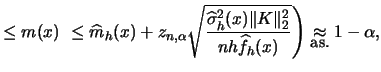
![$\displaystyle \left[\widehat{m}_h (x) - z_{1-\frac{\alpha}{2}} \sqrt{\frac{ \wi...
...{ \widehat{\sigma}_h^2 (x)\Vert K \Vert^2_2 }{nh\widehat{f}_h(x)}}\, \right]\,,$](xlghtmlimg459.gif) |
(6.16) |
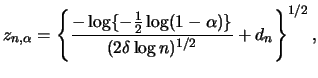
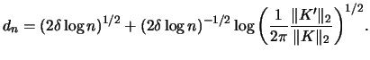
Also similar to the density case, uniform confidence bands for
![]() need rather restrictive assumptions (Härdle; 1990, p. 116).
Suppose that
need rather restrictive assumptions (Härdle; 1990, p. 116).
Suppose that ![]() is a density on
is a density on ![]() and
and
![]() ,
,
![]() . Then it holds under some regularity
for all
. Then it holds under some regularity
for all
![]() :
:
 | |||
 |
|||
Pointwise confidence intervals and uniform confidence bands
using the WARPing approximation are provided by
regci
and
regcb
, respectively. The equivalents for exact
computations are
regxci
and
regxcb
.
The functions
regcb
and
regxcb
can be
directly applied to the original data
![]() ,
the transformation to
,
the transformation to ![]() is performed internally.
The following quantlet code extends the above regression
function by confidence intervals and confidence bands:
is performed internally.
The following quantlet code extends the above regression
function by confidence intervals and confidence bands:
  {mh,mli,mui}=regci(nicfoo,0.18)  ; intervals
  {mh,mlb,mub}=regcb(nicfoo,0.18)  ; bands
  mh =setmask(mh,"line","blue","thick")
  mli=setmask(mli,"line","blue","thin","dashed")
  mui=setmask(mui,"line","blue","thin","dashed")
  mlb=setmask(mlb,"line","blue","thin")
  mub=setmask(mub,"line","blue","thin")
  plot(mh,mli,mui,mlb,mub)
  setgopt(plotdisplay,1,1,"title","Confidence Intervals & Bands")
![\includegraphics[scale=0.425]{smootherrcb}](xlghtmlimg466.gif)
|
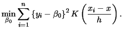
Note that the Nadaraya-Watson estimator is a local constant estimator, i.e. the solution of
The functions
lpregest
and
lpregxest
for local polynomial
regression have essentially the same input as their Nadaraya-Watson
equivalents, except that an additional parameter ![]() to specify the
degree of the polynomial can be given. For local polynomial
regression, an odd value of
to specify the
degree of the polynomial can be given. For local polynomial
regression, an odd value of ![]() is recommended since odd-order
local polynomial regressions outperform even-order local polynomial
regressions.
is recommended since odd-order
local polynomial regressions outperform even-order local polynomial
regressions.
Derivatives of regression functions are computed with
lpderest
or
lpderxest
.
For derivative estimation a polynomial order whose
difference to the derivative order is odd should be used.
Typically one uses the ![]() (local linear) for the estimation
of the regression function and
(local linear) for the estimation
of the regression function and ![]() (local quadratic) for the
estimation of its first derivative.
(local quadratic) for the
estimation of its first derivative.
lpdregxest
and
lpderxest
use automatically
local linear and local quadratic estimation if no order is
specified. The default kernel function is the Quartic kernel
"qua". Appropriate bandwidths can be found by means
of rule of thumbs that replace the unknown regression function
by a higher-order polynomial (Fan and Gijbels; 1996). The following
quantlet code estimates the regression function and its first
derivative by the local polynomial method. Both functions
and the data are plotted together in Figure 6.12.
  motcyc=read("motcyc")
  hh=lpregrot(motcyc)     ; rule-of-thumb bandwidth
  hd=lpderrot(motcyc)     ; rule-of-thumb bandwidth
  mh=lpregest(motcyc,hh)  ; local linear regression
  md=lpderest(motcyc,hd)  ; local quadratic derivative
  mh=setmask(mh,"line","black")
  md=setmask(md,"line","blue","dashed")
  xy=setmask(motcyc,"cross","small","red")
  plot(xy,mh,md)
  setgopt(plotdisplay,1,1,"title","Local Polynomial Estimation")
![\includegraphics[scale=0.425]{smootherreg1}](xlghtmlimg430.gif)
![\includegraphics[scale=0.425]{smootherreg2}](xlghtmlimg431.gif)

![\includegraphics[scale=0.45]{smootherregcv}](xlghtmlimg455.gif)
![\includegraphics[scale=0.425]{smootherlld}](xlghtmlimg478.gif)