10.2 Kalman Filtering and Smoothing

fy = kfilter (y, mu, Sig, H, F, Q, R)

provides Kalman filtering of a (multivariate) time series

sy = ksmoother (y, mu, Sig, H, F, Q, R)

provides Kalman smoothing of a (multivariate) time series

The state-space model consists of two processes -- an observation process $\{y_t \}_{t \in T}$ and an unobservable state process $\{x_t \}_{t \in T}$. Having a sampling of observations made up to time $k$, denoted as $Y_k= \{ y_1, \dots, y_k \}$, we want to find the best estimate of the state $x_t$ that we denote as $\widehat{x}_{t \mid k}$. The particular error covariance matrix is then denoted $P_{t \mid k} = (x_t - \widehat{x}_{t \mid k}) (x_t - \widehat{x}_{t \mid k})^T$. Three different problems are recognized due to different relations between $t$ and $k$:

• Prediction, i.e. estimating $x_t$ in terms of $y_1, \dots, \ y_{t-1}$ (i.e. $k=t-1$).
• Filtering, i.e. estimating $x_t$ in terms of $y_1, \dots, \ y_t$ (i.e. $k=t$).
• Smoothing, i.e. estimating $x_t$ in terms of all observations $y_1, \dots, \ y_T$ (i.e. $k=T$).

To determine the best estimate, the Kalman filtering approach uses the mean squared error (MSE) criterion given as $E (x_t - \widehat{x}_{t \mid k})^T (x_t - \widehat{x}_{t \mid k})$. According to this criterion the best estimate is the conditional expectation $\widehat{x}_{t \mid k}=E (x_t \mid Y_k)$. This expectation is generally nonlinear (and usually difficult to find) and therefore we confine ourselves to linear filters. Since we assume the orthogonality of $(v_t^T, w_t^T)^T$ we are able to derive the desired best linear estimate using techniques of projections onto Hilbert space generated by the observations $Y_k$.

As a result we get the Kalman filter equations

$$\ \widehat{x}_{t \mid t} = \widehat{x}_{t \mid t-1} + P_{t \mid t-1} H^T \ \Delta_t^{-1} (y_t-H \widehat{x}_{t \mid t-1}),$$

$$\ P_{t \mid t} = P_{t \mid t-1} - P_{t \mid t-1} H^T \Delta_t^{-1} H \ P_{t \mid t-1}^T,$$

where $\Delta_t = H P_{t \mid t-1} H^T + Q$, the Kalman prediction equations

$$\ \widehat{x}_{t+1 \mid t} = F \widehat{x}_{t \mid t-1} + \ K_t (y_t - H \widehat{x}_{t \mid t-1}),$$

$$\ P_{t+1 \mid t} = F ( \ P_{t \mid t-1} - P_{t \mid t-1} H^T \Delta_t^{-1} H P_{t \mid t-1} ) F^T + R,$$

and the Kalman smoothing equations

$$\widehat{x}_{t \mid T} = \widehat{x}_{t \mid t} + P_t^* (\widehat{x}_{t+1 \mid T} - F \widehat{x}_{t \mid t}),$$

$$P_{t \mid T} = P_{t \mid t} - P_t^* (P_{t+1 \mid T}-P_{t+1 \mid t}) {P_t^*}^T,$$

$$P_t^* = P_{t \mid t} F^T P_{t+1 \mid t}^{-1}.$$

The matrix $K_t = F P_{t \mid t-1} H^T \Delta_t^{-1}$ is called a gain matrix. Please note that the easy connection between the first two recursions is given by the equation

$$\widehat{x}_{t \mid t-1} = F \widehat{x}_{t-1 \mid t-1}$$

and that the smoothing recursion consists of the backward recursion that uses the filtered values of $x$ and $P$.

Several remarks should be made about the Kalman filter equations. First the inversion of $\Delta_t$ may be replaced with a pseudoinversion. This is generally the case in models with $Q$ singular. Next, the Kalman filter is a minimum square error estimator among all linear estimators but in the case of a Gaussian model it is the minimum square error estimator among all estimators and ${\cal L}(x_t \mid Y_k) = N(\widehat{x}_{t \mid k}, P_{t \mid k})$, i.e. the Kalman filter yields the whole information about the conditional distribution of $x_t$ (this, however, does not hold in a general non-Gaussian model where the Kalman filter yields only information about the first two moments of the conditional distribution of $x_t$).

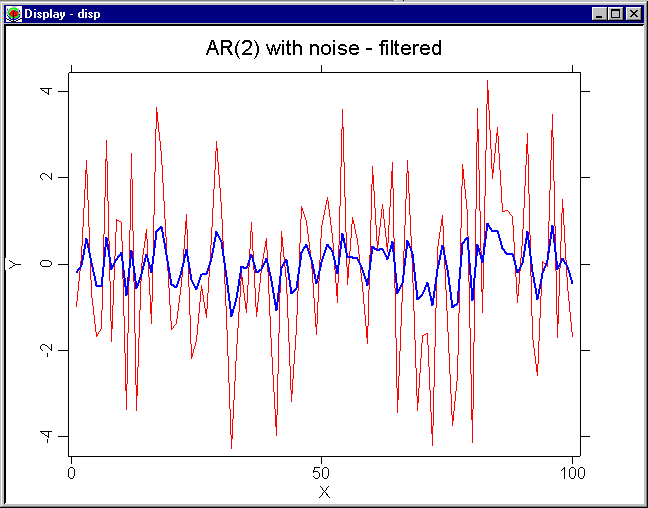
The Kalman filtration equations are implemented in the quantlet kfilter . The input parameters of this quantlet are the time series to be filtered (possibly multivariate), and the system matrices of the underlying state-space model. To filtrate the time series ar2 simulated in the first example type the following instructions.

  x0 = #(0,0)
  Sig = #(0,0)~#(0,0)
  H = 1~0
  F = #(0.5,1)~#(-0.3,0)
  Q = 4
  R = #(1,0)~#(0,0)
  filtered = kfilter(ar2,x0,Sig,H,F,Q,R)

XLGkalm02.xpl

The filtered series is in the variable filtered and the result may be visualized as follows:

  library("plot")
  orig = vec(1:T)~ar2
  filt = vec(1:T)~filtered
  orig = setmask(orig, "line", "red", "thin")
  filt = setmask(filt, "line", "blue", "medium")
  disp = createdisplay(1,1)
  show(disp,1,1, orig, filt)
  setgopt(disp,1,1, "title", "AR(2) with noise - filtered")

XLGkalm02.xpl

The generated series is plotted as a thin red line while the filtered series is plotted as a medium blue line.

The quantlet kfilter saves the file KFOutPut.dat into the XploRe working directory. This file contains all filtered state estimates $x_{t \mid t}$ and their error covariance matrices $P_{t \mid t}$ and might be used to track the development of the estimations' errors or for prediction purposes.

The matrices $P_{t \mid t}$ are vectorized and appended to the state estimation but each of them may be easily recovered. The values of $x_{50 \mid 50}$ and $P_{50 \mid 50}$ might be recovered in the following way:

  KFOutPut = read("KFOutPut.dat")
  dimX = rows(x0)
  x50 = (KFOutPut[50,1:dimX])'
  P50 = reshape(KFOutPut[50,dimX+1:dimX+dimX^2],#(dimX,dimX))

Kalman smoothing equations are implemented by the quantlet ksmoother . Its usage is similar to the quantlet kfilter . Input parameters consist of the time series to be smoothed (possibly multivariate) and the system matrices of the underlying state-space model. In the following sample code the time series ar2 is smoothed and the result is visualized.

  smoothed = ksmoother(ar2,x0,Sig,H,F,Q,R)  
  smoot = vec(1:T)~smoothed
  smoot = setmask(smoot, "line", "blue", "medium")
  disp = createdisplay(1,1)
  show(disp,1,1, orig, smoot)
  setgopt(disp,1,1, "title", "AR(2) with noise - smoothed")

XLGkalm03.xpl

The quantlet ksmoother uses the file KFOutPut.dat during the backward recursions. It generates the file KSOutPut and saves it into the XploRe working directory. Again, this file might be used for analytical purposes.