10.3 Alternating conditional expectations

Breaking down an intricate regression with many variables into a system of simpler relationships - each involving fewer variables - is a desirable goal when modeling high dimensional regression data. Leontief (1947a), for example, considers the process of steel production and points out that the various materials involved in the production of steel should be combined into additional, intermediate variables. Such a goal can be achieved, for instance, by an additive model in which the multivariate regression function $m(x)$ splits up into a sum of nonparametric functions.

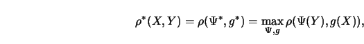
More precisely, let $\Psi ( Y), g_1(X_1), \ldots, g_d(X_d)$ be arbitrary measurable mean zero functions of the corresponding random variables. The fraction of variance not explained by a regression of $\Psi(Y)$ on $\sum_{j=1}^d g_j(X_j)$ is

$$e^2(\Psi, g_1, \ldots, g_d)={E\{[ \Psi(Y) - \sum_{j=1}^d g_j (X_j)]^2\} \over E\Psi^2(Y)}\cdotp$$ (10.3.5)

Define the optimal transformations $\Psi^*, g_1^*, \ldots, g_d^*$ as minimizers of 10.3.5. Such optimal transformations exist and the ACE algorithm (Breiman and Friedman 1985) gives estimates of these transformations. Leontief (1947b) calls such a model additive separable and describes a method of checking this additive separability.

For the bivariate case ($d=1$) the optimal transformations $\Psi^*$ and $g^*$ satisfy

$$\rho^*(X, Y) = \rho(\Psi^*, g^*) = \max_{\Psi,g} \rho(\Psi(Y), g(X)),$$

where $\rho$ is the correlation coefficient. The quantity $\rho^*$ is also known as the maximal correlation coefficient between $X$ and $Y$ and is used as a general measure of dependence. For theoretical properties of maximal correlation I refer to Breiman and Friedman (1985). These authors also report that according to Kolmogorov if $(Y, X_1, \ldots, X_d)$ are jointly normally distributed then the transformations $\Psi, g_j$ having maximal correlation are linear.

Suppose that the data are generated by the regression model

$$\Psi(Y) = \sum_{j=1}^d g_j (X_j) + \varepsilon.$$

Note that the optimal transformations do not correspond to the conditional mean function here. Looking for functions that maximize correlation is not the same as estimating the conditional mean function. However, if the $g_j (X_j)$ have a joint normal distribution and $\varepsilon$ is an independent normal random variable then the optimal transformations are exactly the (linear) transformations $\Psi$ and $g_j$. In general, though, for a regression model of this form with $\varepsilon$ independent of $X$, the optimal transformations are different from the transformations used to construct the model. In practice, the transformations found by the ACE algorithm are sometimes different, as will be seen in the Exercises.

To illustrate the ACE algorithm consider first the bivariate case:

$$e^2(\Psi, g) = E[ \Psi(Y) - g(X)]^2\ .$$ (10.3.6)

The optimal $\Psi(Y)$ for a given $g(X),$ keeping $E\Psi^2(Y)=1$, is

$$\Psi_1(Y)=E[ g(X)\vert Y]\ /\Vert E[ g(X)\vert Y] \Vert,$$ (10.3.7)

with $\Vert \cdot \Vert = [ E(\cdot )^2]^{1/2}$. The minimization of 10.3.6 with respect to $g(X)$ for given $\Psi(Y)$ gives

$$g_1(X) = E[ \Psi(Y) \vert X].$$ (10.3.8)

The basis of the following iterative optimization algorithm is the alternation between the conditional expectations 10.3.7 and 10.3.8.

Algorithm 10.3.1
Basic ace

SET $\Psi(Y) = Y/\Vert Y\Vert;$

REPEAT $g_1(X) = E[ \Psi(Y)\vert X];$

Replace $g(X)$ with $g_1(X);$

$\Psi_1(Y) = E[ g(X)\vert Y] / \Vert E[ g(X)\vert Y] \Vert$

Replace $\Psi(Y)$ with $\Psi_1(Y)$

UNTIL $e^2(\Psi, g)$ fails to decrease.

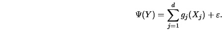
The more general case of multiple predictors can be treated in direct analogy with the basic ACE algorithm. For a given set of functions $\{ g_j(X_j)\}_{j=1}^d$ minimization of 10.3.5, with respect to $\Psi(Y)$, holding $E\Psi^2(Y) =1, \break E\Psi=E g_1= \cdots = E g_d =0$, yields

$$\Psi_1(Y) = E\left[ \sum_{j=1}^d g_j(X_j) \vert Y\right] \big... ...t\Vert E\left[ \sum_{j=1}^d g_j(X_j)\vert Y\right] \right\Vert.$$

Next 10.3.5 is minimized with respect to a single function $g_k(X_k)$ for given $\Psi(Y)$ and given $g_1(X_1), \ldots, g_{k-1}(X_{k-1}), g_{k+1}(X_{k+1}), \ldots, g_d(X_d).$ This iterative procedure is described in the full ACE algorithm.

Algorithm 10.3.2
Full ace

SET $\Psi(Y)=Y/\Vert Y\Vert$ and $g_j(X_j)=0, \quad 1\le j\le d;$

REPEAT

REPEAT

FOR $k=1$ TO $d$ DO BEGIN

$g_{k,1}(X_k) = E[ \Psi(Y)-\sum_{j\ne k} g_j (X_j)\vert X_k];$

$g_k(X_k) = g_{k,1}(X_k);$

END;

UNTIL $e^2(\Psi, g_1, \ldots, g_d)$ fails to decrease;

$\Psi_1(Y)=E[ \sum_{j=1}^d g_j(X_j)\vert Y] / \Vert E[ \sum_{j=1}^d g_j(X_j)\vert Y] \Vert;$

$\Psi(Y)=\Psi_1(Y);$

UNTIL $e^2(\Psi, g_1, \ldots, g_d)$ fails to decrease.

In practice, one has to use smoothers to estimate the involved conditional expectations. Use of a fully automatic smoothing procedure, such as the supersmoother, is recommended. Figure 10.9 shows a three-dimensional data set $(X_1, X_2, Y)$ with $X_1, X_2$ independent standard normals and

$$Y=(X_1+X_2)^3 +\varepsilon,$$

with standard normal errors $\varepsilon.$ The ACE algorithm produced the transformation $g_1$ presented in Figure 10.10.

Figure 10.9: A simulated data set. $X_1,X_2, \varepsilon$ independent standard normal, $Y_i=(X_{i1}+X_{i2})^3+ \varepsilon_i, 1 \leq i \leq n=100$. Made with XploRe (1989).

Figure 10.10: The estimated ACE transformation $g_1 (X_1)$. Made with XploRe (1989).

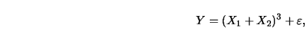
The estimated transformation is remarkably close to the transformation $g_1(x_1)=x_1$. Figure 10.11 displays the estimated transformation $\Psi$, which represents the function $\Psi(y)=y^{1/3}$ extremely well.

Figure 10.11: The estimated transformation $\psi (Y)$. Made with XploRe (1989).

Breiman and Friedman (1985) applied the ACE methodology also to the Boston housing data set (Harrison and Rubinfeld 1978; and Section 10.1). The resulting final model involved four predictors and has an $e^2$ of $0.89$. (An application of ACE to the full 13 variables resulted only in an increase for $e^2$ of $0.02$.) Figure 10.12a shows a plot from their paper of the solution response surface transformation $\Psi(y)$. This function is seen to have a positive curvature for central values of $y$, connecting two straight line segments of different slope on either side. This suggests that the log-transformation used by Harrison and Rubinfeld (1978) may be too severe. Figure 10.12b shows the response transformation for the original untransformed census measurements. The remaining plot in Figure 10.12 display the other transformation $g_j$; for details see Breiman and Friedman (1985).

Figure 10.12: The ACE method applied to the Boston housing data set. (a) Transformed $\log(MV)$; (b) Transformed $M$; (c) Transformed $RM^2$; (d) Transformed $\log(LSTAT)$; (e) Transformed $PT Ratio$; (f) Transformed $Tax$; (g) Transformed $NOX^2$ ; (h) Transformed $y$ versus predictor of transformed $Y$. From Breiman and Friedman (1985) with permission of the American Statistical Association.

Exercises

10.3.1Prove that in the bivariate case the function given in 10.3.7 is indeed the optimal transformation $\Psi^*$.

10.3.2Prove that in the bivariate case the function given in 10.3.8 is indeed the optimal transformation $g^*$.

10.3.3Try the ACE algorithm with some real data. Which smoother would you use as an elementary building block?

10.3.4In the discussion to the Breiman and Friedman article D. Pregibon and Y. Vardi generated data from

$$Y = X_1 X_2$$

with $X_1 \sim U(-1, 1)$ and $X_2 \sim U(0, 1)$. What are possible transformations $\Psi, g$?

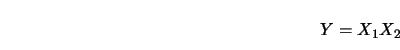
10.3.5Try the ACE algorithm with the data set from Exercise 10.3.2. What transformations do you get? Do they coincide with the transformations you computed in 10.3.2?

[Hint: See the discussion of Breiman and Friedman (1985).]