2.1 Elementary Operations

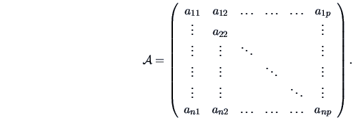
A matrix ${\data{A}}$ is a system of numbers with $n$ rows and $p$ columns:

$${{\data{A}}} = \left (\begin{array}{cccccc} a_{11}&a_{12}&\l... ..._{n1}&a_{n2}&\ldots &\ldots &\ldots &a_{np}\end{array}\right ).$$

We also write $(a_{ij})$ for ${\data{A}}$ and ${\data{A}}(n\times p)$ to indicate the numbers of rows and columns. Vectors are matrices with one column and are denoted as $x$ or $x(p\times 1)$. Special matrices and vectors are defined in Table 2.1. Note that we use small letters for scalars as well as for vectors.

Matrix Operations

Elementary operations are summarized below:

$$\begin{eqnarray*} {\data{A}}^{\top} &=& (a_{ji})\\ {\data{A}}+{\data{B}} &=& (a... ...\data{C}}(n\times m) = \left (\sum^p_{j=1} a_{ij}b_{jk}\right ). \end{eqnarray*}$$

Properties of Matrix Operations

$$\begin{eqnarray*} \data{A}+\data{B} & =& \data{B}+\data{A}\\ \data{A}(\data{B}+... ...\data{A}\\ (\data{A}\data{B})^\top&=&\data{B}^\top\data{A}^\top \end{eqnarray*}$$

Table 2.1: Special matrices and vectors.

Name	Definition	Notation	Example
scalar	$p=n=1$	$a$	3
column vector	$p=1$	$a$	$\left(\begin{array}{c} 1\\ 3\end{array}\right)$
row vector	$n=1$	$a^{\top}$	$\left(\begin{array}{cc} 1\quad 3\\ \end{array} \right)$
vector of ones	$(\underbrace{1,\ldots ,1}_{n})^{\top}$	$1_{n}$	$\left (\begin{array}{c} 1\\ 1 \end{array}\right )$
vector of zeros	$(\underbrace{0,\ldots ,0}_{n})^{\top}$	$0_{n}$	$\left (\begin{array}{c} 0\\ 0 \end{array}\right )$
square matrix	$n=p$	${\data{A}}(p\times p)$	$\left(\begin{array}{cc}2\quad 0\\ 0\quad 2\end{array}\right)$
diagonal matrix	$a_{ij}=0$, $i\not=j$, $n=p$	$\mathop{\hbox{diag}}(a_{ii})$	$\left (\begin{array}{cc}1\quad 0\\ 0\quad 2\end{array}\right )$
identity matrix	$\mathop{\hbox{diag}}(\underbrace{1,\ldots ,1}_{p})$	${\data{I}}_p$	$\left (\begin{array}{cc} 1\quad 0\\ 0\quad 1\end{array}\right)$
unit matrix	$a_{ij}\equiv 1$, $n=p$	$1_{n}1_{n}^{\top}$	$\left (\begin{array}{lll} 1\quad 1\\ 1\quad 1\end{array}\right)$
symmetric matrix	$a_{ij}=a_{ji}$		$\left (\begin{array}{cc} 1\quad 2\\ 2\quad 3\end{array}\right)$
null matrix	$a_{ij}=0$	0	$\left (\begin{array}{cc} 0\quad 0\\ 0\quad 0\end{array}\right)$
upper triangular matrix	$a_{ij}=0, i<j$		$\left (\begin{array}{ccc} 1\quad 2\quad 4\\ 0\quad 1\quad 3\\ 0\quad 0\quad 1\end{array}\right )$
idempotent matrix	${\data{A}\data{A}}={\data{A}}$		${\left ( \begin{array}{rrr} 1 & 0 & 0 \\ 0 & \frac{1}{2} & \frac{1}{2}\\ 0 & \frac{1}{2} & \frac{1}{2} \end{array} \right )}$
orthogonal matrix	${\data{A}}^{\top}{\data{A}}={\data{I}}={\data{A}}{\data{A}}^{\top}$		${\left (\begin{array}{rr}\frac{1}{\sqrt 2} & \frac{1}{\sqrt 2}\\ \frac{1}{\sqrt 2} & -\frac{1}{\sqrt 2} \end{array} \right )}$

Matrix Characteristics

Rank

The rank, $\mathop{\rm {rank}}({\data{A}})$, of a matrix $\data{A}(n\times p)$ is defined as the maximum number of linearly independent rows (columns). A set of $k$ rows $a_j$ of $\data{A}(n\times p)$ are said to be linearly independent if $\sum_{j=1}^k c_j a_j=0_p$ implies $c_j=0, \forall j$, where $c_1,\dots,c_k$ are scalars. In other words no rows in this set can be expressed as a linear combination of the $(k-1)$ remaining rows.

Trace

The trace of a matrix is the sum of its diagonal elements

$$\mathop{\hbox{tr}}({\data{A}}) = \sum ^p_{i=1}a_{ii}.$$

Determinant

The determinant is an important concept of matrix algebra. For a square matrix ${\data A}$, it is defined as:

$$\mathop{\rm {det}}({\data{A}}) = \vert{\data{A}}\vert=\sum (-1)^{\vert\tau \vert}\ a_{1\tau (1)} \ldots a_{p\tau (p)},$$

the summation is over all permutations $\tau$ of $\{1,2,\ldots ,p\}$, and $\vert\tau\vert=0$ if the permutation can be written as a product of an even number of transpositions and $\vert\tau\vert=1$ otherwise.

EXAMPLE 2.1   In the case of $p=2$, ${\data{A}}=\left (\begin{array}{ll} a_{11}&a_{12}\\ a_{21}&a_{22}\end{array}\right)$ and we can permute the digits ``1'' and ``2'' once or not at all. So,

$$\vert{\data{A}}\vert=a_{11}\ a_{22}-a_{12}\ a_{21}.$$

Transpose

For $\data{A}(n\times p)$ and $\data{B}(p \times n)$

$$({\data{A}}^{\top})^{\top}={\data{A}},\textrm{ and }({\data{A}}{\data{B}})^{\top}={\data{B}}^{\top}{\data{A}}^{\top}.$$

Inverse

If $\vert{\data{A}}\vert\not=0$ and ${\data{A}}(p\times p)$, then the inverse ${\data{A}}^{-1}$ exists:

$${\data{A}}\ {\data{A}}^{-1} = {\data{A}}^{-1}\ {\data{A}} = {\data{I}}_p.$$

For small matrices, the inverse of ${\data{A}}=(a_{ij})$ can be calculated as

$${\data{A}}^{-1}=\frac{{\data{C}}}{\vert\data{A}\vert},$$

where ${\data{C}}=(c_{ij})$ is the adjoint matrix of ${\data{A}}$. The elements $c_{ji}$ of ${\data{C}}^{\top}$ are the co-factors of ${\data{A}}$:

$$c_{ji}=(-1)^{i+j}\left\vert \begin{array}{cccccc} a_{1 1}&\... ...{p (j-1)}&a_{p (j+1)}&\dots&a_{p p}\\ \end{array}\right\vert.$$

G-inverse

A more general concept is the $G$-inverse (Generalized Inverse) $\data{A}^-$ which satisfies the following:

$${\data{A}}\ {\data{A}}^-{\data{A}} = {\data{A}}.$$

Later we will see that there may be more than one $G$-inverse.

EXAMPLE 2.2   The generalized inverse can also be calculated for singular matrices. We have:

$$\left( \begin{array}{ll} 1&0\\ 0&0 \end{array}\right) \left... ...ght) = \left( \begin{array}{ll} 1&0\\ 0&0 \end{array}\right),$$

which means that the generalized inverse of ${\data{A}}=\left( \begin{array}{ll} 1&0\\ 0&0 \end{array}\right)$ is ${\data{A}}^-=\left( \begin{array}{ll} 1&0\\ 0&0 \end{array}\right)$ even though the inverse matrix of ${\data{A}}$ does not exist in this case.

Eigenvalues, Eigenvectors

Consider a ($p \times p$) matrix $\data{A}$. If there exists a scalar $\lambda$ and a vector $\gamma$ such that

$${\data{A}}\gamma=\lambda \gamma,$$ (2.1)

then we call

$$\begin{array}{ll} \lambda &\quad \quad \textrm{an eigenvalue}\\ \gamma &\quad \quad \textrm{an eigenvector.} \end{array}$$

It can be proven that an eigenvalue $\lambda$ is a root of the $p$-th order polynomial $\vert\data{A}-\lambda I_p\vert=0$. Therefore, there are up to $p$ eigenvalues $\lambda_1,\lambda_2,\ldots,\lambda_p$ of $\data{A}$. For each eigenvalue $\lambda_j$, there exists a corresponding eigenvector $\gamma_j$ given by equation (2.1) . Suppose the matrix ${\data{A}}$ has the eigenvalues $\lambda_1,\ldots,\lambda_p$. Let $\Lambda =\mathop{\hbox{diag}}(\lambda_1,\ldots,\lambda_p$).

The determinant $\vert{\data{A}}\vert$ and the trace $\mathop{\hbox{tr}}({\data{A}})$ can be rewritten in terms of the eigenvalues:

$$\vert{\data{A}}\vert = \vert\Lambda\vert = \prod ^p_{j=1}\lambda _j$$ (2.2)

$$\mathop{\hbox{tr}}({\data{A}}) = \mathop{\hbox{tr}}(\Lambda) = \sum ^p_{j=1}\lambda _j.$$ (2.3)

An idempotent matrix ${\data{A}}$ (see the definition in Table 2.1) can only have eigenvalues in $\{0,1\}$ therefore $\mathop{\hbox{tr}}({\data{A}})=\mathop{\rm {rank}}({\data{A}}) =$ number of eigenvalues $\neq 0$.

EXAMPLE 2.3   Let us consider the matrix ${\data{A}}={\left ( \begin{array}{rrr} 1 & 0 & 0 \\ 0 & \frac{1}{2} & \frac{1}{2}\\ 0 & \frac{1}{2} & \frac{1}{2} \end{array} \right )}$. It is easy to verify that ${\data{A}} {\data{A}} = {\data{A}}$ which implies that the matrix ${\data{A}}$ is idempotent.

We know that the eigenvalues of an idempotent matrix are equal to 0 or 1. In this case, the eigenvalues of ${\data{A}}$ are $\lambda_1 = 1$, $\lambda_2=1$, and $\lambda_3=0$ since $\left ( \begin{array}{rrr} 1 & 0 & 0 \\ 0 & \frac{1}{2} & \frac{1}{2}\\ ... ... \end{array} \right) = 1 \left( \begin{array}{r}1\\ 0\\ 0 \end{array} \right)$, $\left ( \begin{array}{rrr} 1 & 0 & 0 \\ 0 & \frac{1}{2} & \frac{1}{2}\\ 0... ...begin{array}{r}0\\ \frac{\sqrt{2}}{2}\\ \frac{\sqrt{2}}{2} \end{array} \right)$, and $\left ( \begin{array}{rrr} 1 & 0 & 0 \\ 0 & \frac{1}{2} & \frac{1}{2}\\ ... ...egin{array}{r}0\\ \frac{\sqrt{2}}{2}\\ -\frac{\sqrt{2}}{2} \end{array} \right)$.

Using formulas (2.2) and (2.3), we can calculate the trace and the determinant of ${\data{A}}$ from the eigenvalues: $\mathop{\hbox{tr}}({\data{A}})=\lambda_1+\lambda_2+\lambda_3=2$, $\vert{\data{A}}\vert= \lambda_1 \lambda_2 \lambda_3 = 0$, and $\mathop{\rm {rank}}({\data{A}})=2$.

Properties of Matrix Characteristics

$\data{A}(n \times n),\;\data{B}(n \times n),\; c \in \mathbb{R}$

$$\mathop{\hbox{tr}}(\data{A}+\data{B}) = \mathop{\hbox{tr}}\data{A} + \mathop{\hbox{tr}}\data{B}$$ (2.4)

$$\mathop{\hbox{tr}}(c\data{A}) = c \,\mathop{\hbox{tr}}\data{A}$$ (2.5)

$$\vert c \data{A}\vert = c^n \vert\data{A}\vert$$ (2.6)

$$\vert\data{AB}\vert = \vert\data{BA}\vert = \vert\data{A}\vert\vert\data{B}\vert$$ (2.7)

$\data{A}(n \times p),\; \data{B}(p \times n)$

$$\mathop{\hbox{tr}}(\data{A} \cdotp \data{B}) = \mathop{\hbox{tr}}(\data{B} \cdotp \data{A})$$ (2.8)

$$\mathop{\rm {rank}}({\data A}) \leq \min(n,p)$$

$$\mathop{\rm {rank}}({\data A}) \geq 0$$ (2.9)

$$\mathop{\rm {rank}}({\data A}) = \mathop{\rm {rank}}({\data A}^{\top})$$ (2.10)

$$\mathop{\rm {rank}}({\data A^{\top} A}) = \mathop{\rm {rank}}({\data A})$$ (2.11)

$$\mathop{\rm {rank}}({\data A}+{\data B}) \leq \mathop{\rm {rank}}({\data A}) + \mathop{\rm {rank}}({\data B})$$ (2.12)

$$\mathop{\rm {rank}}({\data A}{\data B}) \leq \min\{ \mathop{\rm {rank}}({\data A}),\mathop{\rm {rank}}({\data B})\}$$ (2.13)

$\data{A}(n \times p),\; \data{B}(p \times q),\; \data{C}(q \times n)$

$$\mathop{\hbox{tr}}(\data{ABC}) = \mathop{\hbox{tr}}(\data{BCA})$$

$$= \mathop{\hbox{tr}}(\data{CAB})$$ (2.14)

$$\mathop{\rm {rank}}(\data{ABC}) = \mathop{\rm {rank}}({\data B}) \quad \textrm{ for nonsingular }{\data{A,C}}$$ (2.15)

$\data{A}( p \times p)$

$$\vert\data{A}^{-1}\vert = \vert\data{A}\vert^{-1}$$ (2.16)

$$\mathop{\rm {rank}}({\data A}) = p \quad \textrm{ if and only if }\data{A}\textrm{ is nonsingular.}$$ (2.17)

Summary

$\ast$

The determinant $\vert\data{A}\vert$ is the product of the eigenvalues of $\data{A}$.

$\ast$

The inverse of a matrix $\data{A}$ exists if $\vert\data{A}\vert\neq 0$.

$\ast$

The trace tr$(\data{A})$ is the sum of the eigenvalues of $\data{A}$.

$\ast$

The sum of the traces of two matrices equals the trace of the sum of the two matrices.

$\ast$

The trace tr $(\data{A}\data{B})$ equals tr $(\data{B}\data{A})$.

$\ast$

The rank$({\data{A}})$ is the maximal number of linearly independent rows (columns) of ${\data{A}}$.