Given a sample of ![]() observations of each variable, in such a way
that the information can be referred to time periods (time-series
data) or can be referred to individuals, firms, etc.
(cross-section data), and assuming linearity, the model can be
specified as follows:
observations of each variable, in such a way
that the information can be referred to time periods (time-series
data) or can be referred to individuals, firms, etc.
(cross-section data), and assuming linearity, the model can be
specified as follows:
The right-hand side of (2.1) which includes the
regressors (![]() ), is called the
), is called the
![]() of the regression function, with
of the regression function, with ![]() (
(
![]() ) being the coefficients or parameters of the
model, which are interpreted as marginal effects, that is to say,
) being the coefficients or parameters of the
model, which are interpreted as marginal effects, that is to say,
![]() measures the change of the endogenous variable when
measures the change of the endogenous variable when
![]() varies a unit, maintaining the rest of regressors as
fixed. The error term
varies a unit, maintaining the rest of regressors as
fixed. The error term ![]() constitutes what is called the
constitutes what is called the
![]() of the model.
of the model.
Expression (2.1) reflects ![]() equations, which can be
written in matrix form in the following terms:
equations, which can be
written in matrix form in the following terms:
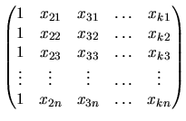 |
(2.3) |
Model (2.2) specifies a causality relationship among
![]() ,
, ![]() and
and ![]() , with
, with ![]() and
and ![]() being considered the factors
which affect
being considered the factors
which affect ![]() .
.
In general terms, model (2.2)(or(2.1)) is
considered as a model of economic behavior where the variable
![]() represents the response of the economic agents to the set of
variables which are contained in
represents the response of the economic agents to the set of
variables which are contained in ![]() , and the error term
, and the error term ![]() contains the deviation to the average behavior.
contains the deviation to the average behavior.