3.3 Proof of Proposition

The proof of this proposition (3.1.1) follows a technique used by Parzen (1962) in the setting of density estimation. Recall the definition of the kernel weights,

$$W_{hi}(x)=K_h(x-X_i)/ \hat f_h(x).$$

Consider the denominator and numerator separately. I show that

$$\hat r_h(x) = n^{-1} \sum^n_{i=1} K_h(x-X_i) Y_i\ {\buildrel p \over \to} \ m(x) f(x)=r(x),$$ (3.3.14)

$$\hat f_h(x) = n^{-1} \sum^n_{i=1} K_h(x-X_i) \ {\buildrel p \over \to} \ f(x).$$ (3.3.15)

From (3.1.9) and (3.3.15) it follows by Slutzky's Theorem Schönfeld (1969, Chapter 6), that

$$\hat r_h(x)/\hat f_hx) \ {\buildrel p \over \to} \ r(x)/f(x) = {m(x)f(x)\over f(x)} = m(x).$$

Only (3.3.14) is shown; the statement (3.3.15) can be proved very similarly. Note that

$$E \hat r_h(x)=\int \int K_h(x-u)y f(u,y) du dy,$$

where $f(u,y)$ denotes the joint density of the distribution of $(X,Y).$ Conditioning on $u$ gives

$$\int K_h(x-u) r(u)du,$$

since

$$m(u) = \int yf(y \vert u) dy = \int yf(u,y) dy/\int f(u,y) dy.$$

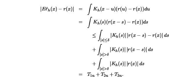
Using integration by substitution it can be shown (see Lemma 3.1 in these Complements) that for $\delta >0$

$$\begin{eqnarray*} \left\vert E \hat r_h(x)-r(x) \right\vert \le & \sup_{\left\ve... ...t s \right\vert \ge \delta/h} \left\vert K(s) \right\vert ds.& \end{eqnarray*}$$

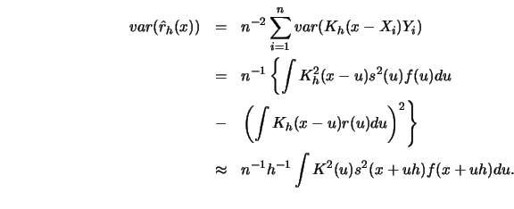
The last two terms of this bound tend to zero, by (A1) and (A2), as $n \to \infty$. Now let $\delta$ tend to zero; then the first term by continuity of $r(\cdot)$ will tend to zero. This proves that $E\hat r_h(x) - r(x) = o(1)$, as $n \to \infty$. Now let $s^2(x)=E(Y^2 \vert X=x)$. Use integration by substitution and the above asymptotic unbiasedness of $\hat r_h(x)$ to see that the variance of $\hat r_h(x)$ is

$$\begin{eqnarray*} var(\hat r_h(x))&=& n^{-2} \sum^n_{i=1} var(K_h(x-X_i) Y_i) \\... ... \\ &\approx& n^{-1} h^{-1} \int K^2(u)s^2(x+uh)f(x+uh)du.\\ \end{eqnarray*}$$

This is asymptotically equal to $n^{-1}h^{-1} \int K^2(u) du$ $s^2(x)f(x)$ using the techniques of splitting up the same integrals as above. Observe now that the variance tends to zero as $nh \to \infty$. This completes the argument since the mean squared error $E(\hat r_h(x)-r(x))^2 = var(\hat r_h(x)) + [E\hat r_h(x)-r(x)]^2 \to 0$ as $n \to \infty,\ nh \to \infty,\ h\to 0$. Thus we have seen that

$$\hat r_h(x) \ {\buildrel 2 \over \to} \ r(x).$$

This implies

$$\hat r_h(x) \ {\buildrel p \over \to} \ r(x),$$

(see Schönfeld; 1969, chapter 6) proof can be adapted to kernel estimation with higher dimensional $X$. If $X$ is $d$-dimensional, change $K_h$ to $h^{-d} K(x/h)$, where $K$: $\mathbb{R}^d\to \mathbb{R}$ and the ratio in the argument of $K$ has to be understood coordinatewise.

LEMMA 3.1   The estimator $\hat r_h(x)$ is asymptotically unbiased as an estimator for $r(x)$.

Use integration by substitution and the fact that the kernel integrates to one to bound

$$\begin{eqnarray*} \left\vert E \hat r_h(x)-r(x) \right\vert &=&\int K_h(x-u)(r(u... ... \left\vert r(x) \right\vert ds\\ &=&T_{1n}+T_{2n}+T_{3n}. \end{eqnarray*}$$

The first term can be bounded in the following way:

$$T_{1n} \le \sup_{\left\vert s \right\vert \le \delta} \left\v... ...r(x-s)-r(x) \right\vert \int \left\vert K(s) \right\vert ds.$$

The third term

$$T_{3n} \le \left\vert r(x) \right\vert \int \left\vert K(s) \right\vert ds.$$

The second term can be bounded as follows:

$$\begin{eqnarray*} T_{2n}&=& \int_{\left\vert s \right\vert > \delta} \left\vert ... ...ft\vert sK(s) \right\vert \int \left\vert r(s) \right\vert ds. \end{eqnarray*}$$

Note that the last integral exists by assumption (A3) of Proposition 3.1.1

3.3.1 Sketch of Proof for Proposition

The derivative estimator $\hat m_h^{(k)}(x)$ is asymptotically unbiased.

$$E\hat m_h^{(k)}(x) = n^{-1} h^{-(k+1)} \sum_{i=1}^n K^{(k)}\left({x-X_i \over h}\right)\ m(X_i)$$ (3.3.16)

$$\approx h^{-k}\ \int K^{(k)}(u)\ m(x-uh) du$$

$$= h^{-k+1}\ \int K^{(k-1)}(u) \ m^{(1)}(x-uh)du$$

$$= \int K(u)\ m^{(k)}(x-uh)du$$

$$\sim m^{(k)}(x) + h^ {d^{(k)}_K} m^{(k+2)}(x)/(k+2)!, \; h \to 0,$$

using partial integration, (A0) and (A4).

The variance of $\hat m_h^{(k)}(x)$ tends to zero if $nh^{2k+1}\to \infty$, as the following calculations show:

$$var\{ \hat m_h^{(k)}(x)\} = n^{-1}h^{-2(k+1)}\,\sum\limits_{i=1}^n \left[ K^{(k)}\ \left({x-X_i\over h}\right) \right]^2 \sigma^2$$ (3.3.17)

$$\approx n^{-1}h^{-2k-1}\ \int [K^{(k)}(u)]^2 du \, \sigma^2.$$