The presented examples clearly show that we not only can, but must use heavy tailed alternatives to the Gaussian law in order to obtain acceptable estimates of market losses. But can we substitute the Gaussian distribution with other distributions in Value at Risk (Expected Shortfall) calculations for whole portfolios of assets? Recall, that the definition of VaR utilizes the quantiles of the portfolio returns distribution and not the returns distribution of individual assets in the portfolio. If all asset return distributions are assumed to be Gaussian then the portfolio distribution is multivariate normal and well known statistical tools can be applied ([45]). However, when asset returns are distributed according to a different law (or different laws!) then the multivariate distribution may be hard to tackle. In particular, linear correlation may no longer be a meaningful measure of dependence.
Luckily for us multivariate statistics offers the concept of copulas,
for a review see [34] and [78].
In rough terms, a copula is a function
![]() with certain special properties. Alternatively we can say that it is
a multivariate distribution function defined on the unit cube
with certain special properties. Alternatively we can say that it is
a multivariate distribution function defined on the unit cube
![]() . The technical definitions of copulas that can be found in
the literature often look more complicated, but to a financial
modeler, this definition is enough to build an intuition from. What
is important for VaR calculations is that a copula enables us to
construct a multivariate distribution function from the marginal
(possibly different) distribution functions of
. The technical definitions of copulas that can be found in
the literature often look more complicated, but to a financial
modeler, this definition is enough to build an intuition from. What
is important for VaR calculations is that a copula enables us to
construct a multivariate distribution function from the marginal
(possibly different) distribution functions of ![]() individual asset
returns in a way that takes their dependence structure into
account. This dependence structure may be no longer measured by
correlation, but by other adequate functions like rank correlation,
comonotonicity and, especially, tail dependence
([91]). Moreover, it can be shown that for every multivariate
distribution function there exists a copula which contains all
information on dependence.
For example, if the random variables are independent, then
the independence copula (also known as the product copula) is just the
product of
individual asset
returns in a way that takes their dependence structure into
account. This dependence structure may be no longer measured by
correlation, but by other adequate functions like rank correlation,
comonotonicity and, especially, tail dependence
([91]). Moreover, it can be shown that for every multivariate
distribution function there exists a copula which contains all
information on dependence.
For example, if the random variables are independent, then
the independence copula (also known as the product copula) is just the
product of ![]() variables:
variables:
![]() . If the random variables have a multivariate normal
distribution with a given covariance matrix then the Gaussian copula
is obtained.
. If the random variables have a multivariate normal
distribution with a given covariance matrix then the Gaussian copula
is obtained.
Copula functions do not impose any restrictions on the model, so in
order to reach a model that is to be useful in a given risk management
problem, a particular specification of the copula must be chosen. From
the wide variety of copulas that exist probably the elliptical and
Archimedean copulas are the ones most often used in
applications. Elliptical copulas are simply the copulas of
elliptically contoured (or elliptical) distributions,
e.g. (multivariate) normal, ![]() , symmetric stable and symmetric
generalized hyperbolic ([38]). Rank correlation and
tail dependence coefficients can be easily calculated for elliptical
copulas. There are, however, drawbacks - elliptical copulas do not
have closed form expressions, are restricted to have radial symmetry
and have all marginal distributions of the same type. These
restrictions may disqualify elliptical copulas from being used in some
risk management problems. In particular, there is usually a stronger
dependence between big losses (e.g. market crashes) than between big
gains. Clearly, such asymmetries cannot be modeled with elliptical
copulas.
In contrast to elliptical copulas, all commonly encountered
Archimedean copulas have closed form expressions. Their popularity
also stems from the fact that they allow for a great variety of
different dependence structures ([41,50]). Many
interesting parametric families of copulas are Archimedean, including
the well known Clayton, Frank and Gumbel copulas.
, symmetric stable and symmetric
generalized hyperbolic ([38]). Rank correlation and
tail dependence coefficients can be easily calculated for elliptical
copulas. There are, however, drawbacks - elliptical copulas do not
have closed form expressions, are restricted to have radial symmetry
and have all marginal distributions of the same type. These
restrictions may disqualify elliptical copulas from being used in some
risk management problems. In particular, there is usually a stronger
dependence between big losses (e.g. market crashes) than between big
gains. Clearly, such asymmetries cannot be modeled with elliptical
copulas.
In contrast to elliptical copulas, all commonly encountered
Archimedean copulas have closed form expressions. Their popularity
also stems from the fact that they allow for a great variety of
different dependence structures ([41,50]). Many
interesting parametric families of copulas are Archimedean, including
the well known Clayton, Frank and Gumbel copulas.
After the marginal distributions of asset returns are estimated and a particular copula type is selected, the copula parameters have to be estimated. The fit can be performed by least squares or maximum likelihood. Note, however, that for some copula types it may not be possible to maximize the likelihood function. In such cases the least squares technique should be used. A review of the estimation methods - including a description of the relevant XploRe quantlets - can be found in [88].
For risk management purposes, we are interested in the Value at Risk
of a portfolio of assets. While analytical methods for the computation
of VaR exist for the multivariate normal distribution (i.e. for the
Gaussian copula), in most other cases we have to use Monte Carlo
simulations. A general technique for random variate generation from
copulas is the conditional distributions method ([78]).
A random vector
![]() having a joint distribution
function
having a joint distribution
function ![]() can be generated by the following algorithm:
can be generated by the following algorithm:
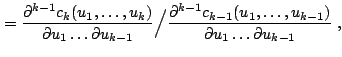 |
 |
Copulas allow us to construct models which go beyond the standard notions of correlation and multivariate Gaussian distributions. As such, in conjunction with alternative asset returns distributions discussed earlier in this chapter, they yield an ideal tool to model a wide variety of financial portfolios and products. No wonder they are gradually becoming an element of good risk management practice.