5.2 Generalized Linear Models

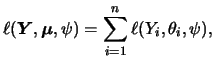
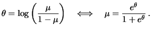
Generalized linear models (GLM) extend the concept of the widely used linear regression model. The linear model assumes that the response $Y$ (the dependent variable) is equal to a linear combination ${\boldsymbol{X}}^\top{\boldsymbol{\beta}}$ and a normally distributed error term:

$$Y ={\boldsymbol{X}}^\top{\boldsymbol{\beta}}+\varepsilon.$$

The least squares estimator $\widehat{{\boldsymbol{\beta}}}$ is adapted to these assumptions. However, the restriction of linearity is far too strict for a variety of practical situations. For example, a continuous distribution of the error term implies that the response $Y$ has a continuous distribution as well. Hence, this standard linear regression model fails, for example, when dealing with binary data (Bernoulli $Y$) or with count data (Poisson $Y$).

Nelder & Wedderburn (1972) introduced the term generalized linear models (GLM). A good resource of material on this model is the monograph of McCullagh & Nelder (1989). The essential feature of the GLM is that the regression function, i.e. the expectation $\mu=E(Y\vert{\boldsymbol{X}})$ of $Y$ is a monotone function of the index $\eta={\boldsymbol{X}}^\top {\boldsymbol{\beta}}$. We denote the function which relates $\mu$ and $\eta$ by $G$:

$$E(Y\vert{\boldsymbol{X}}) = G({\boldsymbol{X}}^\top {\boldsymbol{\beta}})\index{link function} \quad\iff\quad \mu=G(\eta).$$

This function $G$ is called the link function. (We remark that Nelder & Wedderburn (1972), McCullagh & Nelder (1989) actually denote $G^{-1}$ as the link function.)

5.2.1 Exponential Families

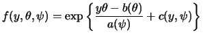
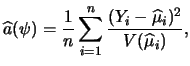
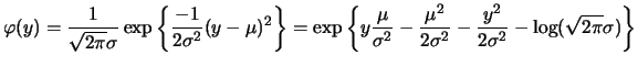
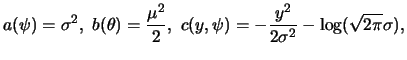
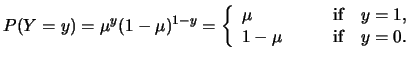
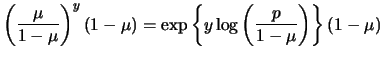
In the GLM framework we assume that the distribution of $Y$ is a member of the exponential family. The exponential family covers a broad range of distributions, for example discrete as the Bernoulli or Poisson distribution and continuous as the Gaussian (normal) or Gamma distribution.

A distribution is said to be a member of the exponential family if its probability function (if $Y$ discrete) or its density function (if $Y$ continuous) has the structure

$$f(y,\theta,\psi) = \exp\left\{\frac{y\theta-b(\theta)}{a(\psi)} + c(y,\psi)\right\}$$ (5.13)

with some specific functions $a(\bullet)$, $b(\bullet)$ and $c(\bullet)$. These functions differ for the distinct $Y$ distributions. Generally speaking, we are only interested in estimating the parameter $\theta$. The additional parameter $\psi$ is -- as the variance $\sigma^2$ in the linear regression -- a nuisance parameter. McCullagh & Nelder (1989) call $\theta$ the canonical parameter.

EXAMPLE 5.2  
Suppose $Y$ is normally distributed, i.e. $Y\sim N(\mu,\sigma^2)$. Hence we can write its density as

$$\varphi(y) = \frac{1}{\sqrt{2\pi}\sigma} \exp\left\{\frac{-1}{2\s... ...c{\mu^2}{2\sigma^2} - \frac{y^2}{2\sigma^2} - \log(\sqrt{2\pi}\sigma) \right\}$$

and we see that the normal distribution is a member of the exponential family with

$$a(\psi) = \sigma^2, \ b(\theta)= \frac{\mu^2}{2}, \ c(y,\psi)= - \frac{y^2}{2\sigma^2} - \log(\sqrt{2\pi}\sigma),$$

where we set $\psi=\sigma$ and $\theta=\mu$. $\Box$

EXAMPLE 5.3  
Suppose now $Y$ is Bernoulli distributed, i.e. its probability function is

$$P(Y=y) = \mu^y (1-\mu)^{1-y} = \left\{\begin{array}{ll} \mu &\qqu... ...textrm{if}\quad y=1,\\ 1-\mu &\qquad \textrm{if}\quad y=0. \end{array}\right.$$

This can be transformed into

$$P(Y=y) = \left(\frac{\mu}{1-\mu}\right)^y (1-\mu) =\exp\left\{y\log\left( \frac{p}{1-\mu}\right)\right\} (1-\mu)$$

using the logit

$$\theta = \log\left( \frac{\mu}{1-\mu}\right) \quad \Longleftrightarrow \quad \mu = \frac{e^\theta}{1+e^\theta}\,.$$

Thus we have an exponential family with

$$a(\psi) = 1, \ b(\theta) = -\log(1-\mu) = \log(1+e^\theta), \ c(y,\psi) \equiv 0.$$

This is a distribution without an additional nuisance parameter $\psi$. $\Box$

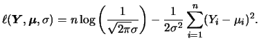
It is known that the least squares estimator $\widehat{{\boldsymbol{\beta}}}$ in the classical linear model is also the maximum-likelihood estimator for normally distributed errors. By imposing that the distribution of $Y$ belongs to the exponential family it is possible to stay in the framework of maximum-likelihood for the GLM. Moreover, the use of the general concept of exponential families has the advantage that we can derive properties of different distributions at the same time.

To derive the maximum-likelihood algorithm in detail, we need to present some more properties of the probability function or density function $f(\bullet)$. First of all, $f$ is a density (w.r.t. the Lebesgue measure in the continuous and w.r.t. the counting measure in the discrete case). This allows us to write

$$\int f(y,\theta,\psi)\,dy=1.$$

Under some suitable regularity conditions (it is possible to exchange differentiation and integration) this yields

$$= \frac{\partial}{\partial\theta} \int f(y,\theta,\psi)\,dy = \int \frac{\partial}{\partial\theta} f(y,\theta,\psi)\,dy$$ 0

$$= \int \left\{\frac{\partial}{\partial\theta} \log f(y,\theta,\psi)... ... \,dy = E\left\{\frac{\partial}{\partial\theta} \ell(y,\theta,\psi) \right\}\,,$$

where $\ell(y,\theta,\psi)$ denotes the log-likelihood, i.e.

$$\ell(y,\theta,\psi)=\log f(y,\theta,\psi).$$ (5.14)

The function $\frac{\partial}{\partial\theta} \ell(y,\theta,\psi)$ is typically called score and it is known that

$$E\left\{ \frac{\partial^2}{\partial\theta^2} \ell(y,\theta,\psi)... ...= -E \left\{ \frac{\partial}{\partial\theta} \ell(y,\theta,\psi) \right\}^2\,.$$

This and taking first and second derivatives of (5.13) gives now

$$0 = E \left\{ \frac{Y-b'(\theta)}{a(\psi)}\right\}, \quad\textrm{... ...heta)}{a(\psi)}\right\} = - E \left\{ \frac{Y-b'(\theta)}{a(\psi)}\right\}^2\,.$$

We can conclude

$$E(Y) = \mu = b'(\theta),$$

$$\mathop{\mathit{Var}}(Y) = V(\mu) a(\psi) = b''(\theta) a(\psi).$$

We observe that the expectation of $Y$ only depends on $\theta$ whereas the variance of $Y$ depends on the parameter of interest $\theta$ and the nuisance parameter $\psi$. Typically one assumes that the factor $a(\psi)$ is identical over all observations.

5.2.2 Link Functions

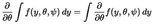Apart from the distribution of $Y$, the link function $G$ is another important part of the GLM. Recall the notation

$$\eta = {\boldsymbol{X}}^\top {\boldsymbol{\beta}}, \ \mu = G(\eta).$$

In the case that

$${\boldsymbol{X}}^\top {\boldsymbol{\beta}}= \eta =\theta$$

the link function is called canonical link function. For models with a canonical link, some theoretical and practical problems are easier to solve. Table 5.2 summarizes characteristics for some exponential functions together with canonical parameters $\theta$ and their canonical link functions. Note that for the binomial and the negative binomial distribution we assume the parameter $k$ to be known. The case of binary $Y$ is a special case of the binomial distribution ($k=1$).

What link functions can we choose apart from the canonical? For most of the models a number of special link functions exist. For binomial $Y$ for example, the logistic or Gaussian link functions are often used. Recall that a binomial model with the canonical logit link is called logit model. If the binomial distribution is combined with the Gaussian link, it is called probit model. A further alternative for binomial $Y$ is the complementary log-log link

$$\eta=\log\{-\log(1-\mu)\}.$$

A very flexible class of link functions is the class of power functions which are also called Box-Cox transformations (Box & Cox, 1964). They can be defined for all models for which we have observations with positive mean. This family is usually specified as

$$\eta = \left\{\begin{array}{ll} \mu^\lambda&\qquad \textrm{if}\quad\lambda\ne 0,\\ \log \mu &\qquad \textrm{if}\quad\lambda=0. \end{array}\right.$$

3pt

Table 5.2: Characteristics of some GLM distributions

Notation	Range			Canonical	Variance
	of $y$	$b(\theta)$	$\mu(\theta)$	link $\theta(\mu)$	$V(\mu)$	$a(\psi)$
Bernoulli $B(\mu)$	$\{0,1\}$	$\log(1+e^\theta)$	$\frac{\displaystyle e^\theta}{\displaystyle 1+e^\theta}$	logit	$\mu(1-\mu)$	1
Binomial $B(k,\mu)$	$[0,k]$ integer	$k\log(1+e^\theta)$	$\frac{\displaystyle ke^\theta}{\displaystyle 1+e^\theta}$	$\log\left(\frac{\displaystyle\mu}{\displaystyle k-\mu}\right)$	$\mu\left(1-\frac{\displaystyle \mu}{\displaystyle k}\right)$	1
Poisson $P(\mu)$	$[0,\infty)$ integer	$\exp(\theta)$	$\exp(\theta)$	$\log$	$\mu$	1
Negative Binomial $N{\!}B(\mu,k)$	$[0,\infty)$ integer	$- k\log(1 - e^{\theta})$	$\frac{\displaystyle ke^\theta\!}{\displaystyle 1-e^\theta}$	$\log\left(\frac{\displaystyle\mu}{\displaystyle k+\mu}\right)$	$\mu + \frac{\displaystyle \mu^2}{\displaystyle k}$	1
Normal $N(\mu,\sigma^2)$	$(-\infty,\infty)$	$\theta^2/2$	$\theta$	identity	1	$\sigma^2$
Gamma $G(\mu,\nu)$	$(0,\infty)$	$-\log(-\theta)$	$-\,1/\theta$	reciprocal	$\mu^2$	$1/\nu$
Inverse Gaussian $IG(\mu,\sigma^2)$	$(0,\infty)$	$-(-2\theta)^{1/2}$	$\frac{\displaystyle -1}{\displaystyle \sqrt{(-2\theta)}}$	squared reciprocal	$\mu^3$	$\sigma^2$

5.2.3 Iteratively Reweighted Least Squares Algorithm

As already pointed out, the estimation method of choice for a GLM is maximizing the likelihood function with respect to ${\boldsymbol{\beta}}$. Suppose that we have the vector of observations ${\boldsymbol{Y}}=(Y_1,\ldots,Y_n)^\top$ and denote their expectations (given ${\boldsymbol{X}}_i={\boldsymbol{x}}_i$) by the vector ${\boldsymbol{\mu}}=(\mu_1,\ldots,\mu_n)^\top$. More precisely, we have

$$\mu_i= G({\boldsymbol{x}}_i^\top {\boldsymbol{\beta}}).$$

The log-likelihood of the vector ${\boldsymbol{Y}}$ is then

$$\ell({\boldsymbol{Y}},{\boldsymbol{\mu}},\psi) = \sum_{i=1}^n \ell(Y_i,\theta_i,\psi),$$ (5.15)

where $\theta_i=\theta(\eta_i)=\theta({\boldsymbol{x}}_i^\top {\boldsymbol{\beta}})$ and $\ell(\bullet)$ on the right hand side of (5.15) denotes the individual log-likelihood contribution for each observation $i$.

EXAMPLE 5.4  
For $Y_i\sim N(\mu_i,\sigma^2)$ we have

$$\ell(Y_i,\theta_i,\psi)=\log\left(\frac{1}{\sqrt{2\pi}\sigma}\right) -\frac {1}{2\sigma^2} (Y_i-\mu_i)^2.$$

This gives the sample log-likelihood

$$\ell({\boldsymbol{Y}},{\boldsymbol{\mu}},\sigma)= n\log\left(\frac{1}{\sqrt{2\pi}\sigma}\right) -\frac {1}{2\sigma^2} \sum_{i=1}^n (Y_i-\mu_i)^2.$$ (5.16)

Obviously, maximizing the log-likelihood for ${\boldsymbol{\beta}}$ under normal $Y$ is equivalent to minimizing the least squares criterion as the objective function. $\Box$

EXAMPLE 5.5  
The calculation in Example 5.3 shows that the individual log-likelihood for the binary responses $Y_i$ equals $\ell(Y_i,\theta_i,\psi)=Y_i\log(\mu_i)+(1-Y_i)\log(1-\mu_i)$. This leads to the sample version

$$\ell({\boldsymbol{Y}},{\boldsymbol{\mu}},\psi)=\sum_{i=1}^n \left\{Y_i\log(\mu_i)+(1-Y_i)\log(1-\mu_i)\right\}.$$ (5.17)

Note that one typically defines $0\cdotp\log(0)=0$. $\Box$

Let us remark that in the case where the distribution of $Y$ itself is unknown, but its two first moments can be specified, then the quasi-likelihood may replace the log-likelihood (5.14). This means we assume that

$$E(Y) = \mu,$$

$$\mathop{\mathit{Var}}(Y) = a(\psi)\,V(\mu).$$

The quasi-likelihood is defined by

$$\ell(y,\theta,\psi) = \frac{1}{a(\psi)} \int\limits^y_{\mu(\theta)} \frac{(s-y)}{V(s)}\,ds\,,$$ (5.18)

cf. Nelder & Wedderburn (1972). If $Y$ comes from an exponential family then the derivatives of (5.14) and (5.18) coincide. Thus, (5.18) establishes in fact a generalization of the likelihood approach.

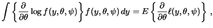
Alternatively to the log-likelihood the deviance is used often. The deviance function is defined as

$$D({\boldsymbol{Y}},{\boldsymbol{\mu}},\psi) = 2 \left\{ \ell({\bo... ...bol{\mu}}^{max},\psi) -\ell({\boldsymbol{Y}},{\boldsymbol{\mu}},\psi) \right\},$$ (5.19)

where ${\boldsymbol{\mu}}^{max}$ (typically ${\boldsymbol{Y}}$) is the non-restricted vector maximizing $\ell({\boldsymbol{Y}},\bullet,\psi)$. The deviance (up to the factor $a(\psi)$) is the GLM analog of the residual sum of squares (RSS) in linear regression and compares the log-likelihood $\ell$ for the ``model'' $\mu$ with the maximal achievable value of $\ell$. Since the first term in (5.19) is not dependent on the model and therefore not on ${\boldsymbol{\beta}}$, minimization of the deviance corresponds exactly to maximization of the log-likelihood.

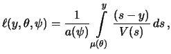
Before deriving the algorithm to determine ${\boldsymbol{\beta}}$, let us have a look at (5.15) again. From $\ell(Y_i,\theta_i,\psi) =\log f(Y_i,\theta_i,\psi)$ and (5.13) we see

$$\ell({\boldsymbol{Y}},{\boldsymbol{\mu}},\psi) = \sum_{i=1}^n \left\{\frac{Y_i\theta_i-b(\theta_i)}{a(\psi)} - c(Y_i,\psi)\right\}.$$ (5.20)

Obviously, neither $a(\psi)$ nor $c(Y_i,\psi)$ have an influence on the maximization, hence it is sufficient to consider

$$\widetilde\ell({\boldsymbol{Y}},{\boldsymbol{\mu}}) = \sum_{i=1}^n \left\{Y_i\theta_i-b(\theta_i)\right\}.$$ (5.21)

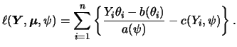
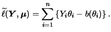
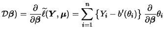
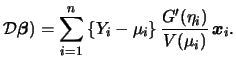
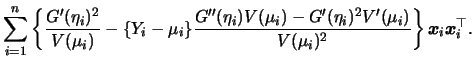
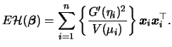
We will now maximize (5.21) w.r.t. ${\boldsymbol{\beta}}$. For that purpose take the first derivative of (5.21). This yields the gradient

$$\CD {\boldsymbol{\beta}}) =\frac{\partial}{\partial{\boldsymbol{\... ...Y_i-b'(\theta_i)\right\} \frac{\partial}{\partial{\boldsymbol{\beta}}} \theta_i$$ (5.22)

and our optimization problem is to solve

$$\CD {\boldsymbol{\beta}}) = 0,$$

a (in general) nonlinear system of equations in ${\boldsymbol{\beta}}$. For that reason, an iterative method is needed. One possible solution is the Newton-Raphson algorithm, a generalization of the Newton algorithm for the multidimensional parameter. Denote ${\mathcal{H}}({\boldsymbol{\beta}})$ the Hessian of the log-likelihood, i.e. the matrix of second derivatives with respect to all components of ${\boldsymbol{\beta}}$. Then, one Newton-Raphson iteration step for ${\boldsymbol{\beta}}$ is

$$\widehat{{\boldsymbol{\beta}}}^{new} = \widehat{{\boldsymbol{\bet... ...dsymbol{\beta}}}^{old}) \right\}^{-1} \CD\widehat{{\boldsymbol{\beta}}}^{old}).$$

A variant of the Newton-Raphson is the Fisher scoring algorithm which replaces the Hessian by its expectation (w.r.t. the observations $Y_i$)

$$\widehat{{\boldsymbol{\beta}}}^{new} = \widehat{{\boldsymbol{\bet... ...dsymbol{\beta}}}^{old}) \right\}^{-1} \CD\widehat{{\boldsymbol{\beta}}}^{old}).$$

To present both algorithms in a more detailed way, we need again some additional notation. Recall that we have $\mu_i=G({\boldsymbol{x}}_i^\top {\boldsymbol{\beta}}) =b'(\theta_i)$, $\eta_i={\boldsymbol{x}}_i^\top {\boldsymbol{\beta}}$ and $b'(\theta_i)=\mu_i=G(\eta_i)$. For the first and second derivatives of $\theta_i$ we obtain (after some calculation)

$$\frac{\partial}{\partial{\boldsymbol{\beta}}} \theta_i = \frac{G'(\eta_i)}{V(\mu_i)} \, {\boldsymbol{x}}_i$$

$$\frac{\partial^2}{\partial{\boldsymbol{\beta}}{\boldsymbol{\beta}}^\top } \theta_i = \frac{G''(\eta_i)V(\mu_i) - G'(\eta_i)^2V'(\mu_i)}{V(\mu_i)^2} \, {\boldsymbol{x}}_i {\boldsymbol{x}}_i^\top .$$

Using this, we can express the gradient of the log-likelihood as

$$\CD {\boldsymbol{\beta}}) = \sum_{i=1}^n \left\{Y_i-\mu_i\right\} \frac{G'(\eta_i)}{V(\mu_i)} \, {\boldsymbol{x}}_i.$$

For the Hessian we get

$${\mathcal{H}}({\boldsymbol{\beta}}) = \sum_{i=1}^n \left\{ -b''(\theta_i) \left(\frac{\partial}{\partia... ...al^2}{\partial{\boldsymbol{\beta}}{\boldsymbol{\beta}}^\top } \theta_i \right\}$$

$$= \sum_{i=1}^n \left\{\frac{G'(\eta_i)^2}{V(\mu_i)} - \{Y_i-\mu_i\}... ...i)^2V'(\mu_i)}{V(\mu_i)^2} \right\}{\boldsymbol{x}}_i {\boldsymbol{x}}_i^\top .$$

Since $EY_i=\mu_i$ it turns out that the Fisher scoring algorithm is easier: We replace ${\mathcal{H}}({\boldsymbol{\beta}})$ by

$$E{\mathcal{H}}({\boldsymbol{\beta}}) = \sum_{i=1}^n \left\{\frac{G'(\eta_i)^2}{V(\mu_i)} \right\}{\boldsymbol{x}}_i {\boldsymbol{x}}_i^\top .$$

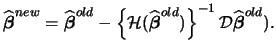
For the sake of simplicity let us concentrate on the Fisher scoring for the moment. Define the weight matrix

$${\mathbf{W}}= \mathop{\hbox{diag}}\left( \frac{G'(\eta_1)^2}{V(\mu_1)},\ldots, \frac{G'(\eta_n)^2}{V(\mu_n)}\right).$$

Additionally, define

$$\widetilde{{\boldsymbol{Y}}} = \left( \frac{Y_1-\mu_1}{G'(\eta_1)},\ldots, \frac{Y_n-\mu_n}{G'(\eta_n)}\right)^\top$$

and the design matrix

$${\mathbf{X}}= \left(\begin{array}{c}{\boldsymbol{x}}_1^\top \\ \vdots\\ {\boldsymbol{x}}_1^\top \end{array} \right).$$

Then one iteration step for ${\boldsymbol{\beta}}$ can be rewritten as

$${\boldsymbol{\beta}}^{new} = {\boldsymbol{\beta}}^{old}+ ({\mathbf{X}}^\top {\mathbf{W}} {\mathbf{X}})^{-1} {\mathbf{X}}^\top {\mathbf{W}} \widetilde{{\boldsymbol{Y}}}$$

$$= ({\mathbf{X}}^\top {\mathbf{W}}{\mathbf{X}})^{-1} {\mathbf{X}}^\top {\mathbf{W}}{{\boldsymbol{Z}}}$$ (5.23)

where ${\boldsymbol{Z}}=(Z_1,\ldots,Z_n)^\top$ is the vector of adjusted dependent variables

$$Z_i= {\boldsymbol{x}}_i^\top {\boldsymbol{\beta}}^{old} + (Y_i-\mu_i) \{G'(\eta_i)\}^{-1}.$$ (5.24)

The iteration stops when the parameter estimate or the log-likelihood (or both) do not change significantly any more. We denote the resulting parameter estimate by $\widehat{\boldsymbol{\beta}}$.

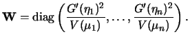
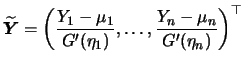
We see that each iteration step (5.23) is the result of a weighted least squares regression on the adjusted variables $Z_i$ on ${\boldsymbol{x}}_i$. Hence, a GLM can be estimated by iteratively reweighted least squares (IRLS). Note further that in the linear regression model, where we have $G'\equiv 1$ and $\mu_i=\eta_i={\boldsymbol{x}}_i^\top {\boldsymbol{\beta}}$, no iteration is necessary. The Newton-Raphson algorithm can be given in a similar way (with the more complicated weights and a different formula for the adjusted variables). There are several remarks on the algorithm:

• In the case of a canonical link function, the Newton-Raphson and the Fisher scoring algorithm coincide. Here the second derivative of $\theta_i$ is zero.

  Additionally we have

  $$b'(\theta_i)=G(\theta_i) \quad \Longrightarrow\quad b''(\theta_i)=G'(\theta_i)=V(\mu_i).$$
  This also simplifies the weight matrix ${\mathbf{W}}$.
• We still have to address the problem of starting values. A naive way would be just to start with some arbitrary ${\boldsymbol{\beta}}_{0}$, as e.g. ${\boldsymbol{\beta}}_{0}=0$. It turns out that we do not in fact need a starting value for ${\boldsymbol{\beta}}$ since the adjusted dependent variable can be equivalently initialized by appropriate $\eta_{i,0}$ and $\mu_{i,0}$. Typically the following choices are made, we refer here to McCullagh & Nelder (1989).
  • For all but binomial models:
    $\mu_{i,0}=Y_i$ and $\eta_{i,0}=G^{-1}(\mu_{i,0})$
  • For binomial models:
    $\mu_{i,0}=(Y_i+\frac{1}{2})/(k+1)$ and $\eta_{i,0}=G^{-1}(\mu_{i,0})$.
    ($k$ denotes the binomial weights, i.e. $k=1$ in the Bernoulli case.)
• An estimate $\widehat\psi$ for the dispersion parameter $\psi$ can be obtained from

  $$\widehat{a}(\psi) = \frac{1}{n} \sum\limits^n_{i=1} \frac{(Y_i - \widehat{\mu}_i)^2}{V(\widehat{\mu}_i)},$$ (5.25)

  
  
  when $\widehat{\mu}_i$ denotes the estimated regression function for the $i$th observation.

The resulting estimator $\widehat{{\boldsymbol{\beta}}}$ has an asymptotic normal distribution, except of course for the standard linear regression case with normal errors where $\widehat{{\boldsymbol{\beta}}}$ has an exact normal distribution.

THEOREM 5.1  
Under regularity conditions and as $n\to\infty$ we have for the estimated coefficient vector

$$\sqrt{n} (\widehat{{\boldsymbol{\beta}}} - {\boldsymbol{\beta}}) \mathrel{\mathop{\longrightarrow}\limits_{}^{L}} N(0,{\mathbf{\Sigma}}).$$

Denote further by $\widehat{{\boldsymbol{\mu}}}$ the estimator of ${\boldsymbol{\mu}}$. Then, for deviance and log-likelihood it holds approximately: $D({\boldsymbol{Y}},\widehat{{\boldsymbol{\mu}}},\psi)\sim \chi^2_{n-d}$ and $2\{\ell({\boldsymbol{Y}},\widehat{{\boldsymbol{\mu}}},\psi)-\ell({\boldsymbol{Y}},{{\boldsymbol{\mu}}},\psi)\}\sim\chi^2_{d}$.

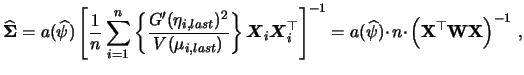
The asymptotic covariance of the coefficient $\widehat{{\boldsymbol{\beta}}}$ can be estimated by

$$\widehat{{\mathbf{\Sigma}}} = a(\widehat\psi)\left[ \frac1n\sum_{... ...)\cdotp n \cdotp \left({\mathbf{X}}^\top{\mathbf{W}}{\mathbf{X}}\right)^{-1}\,,$$

with the subscript ${last}$ denoting the values from the last iteration step. Using this estimated covariance we can make inference about the components of ${\boldsymbol{\beta}}$ such as tests of significance. For selection between two nested models, typically a likelihood ratio test (LR test) is used.

EXAMPLE 5.6  
Let us illustrate the GLM using the data on East-West German migration from Table 5.1. This is a sample of East Germans who have been surveyed in 1991 in the German Socio-Economic Panel, see GSOEP (1991). Among other questions the participants have been asked if they can imagine moving to the Western part of Germany or West Berlin. We give the value 1 for those who responded positively and 0 if not.

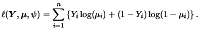
Recall that the economic model is based on the idea that a person will migrate if the utility (wage differential) exceeds the costs of migration. Of course neither one of the variables, wage differential and costs, are directly available. It is obvious that age has an important influence on migration intention. Younger people will have a higher wage differential. A currently low household income and unemployment will also increase a possible gain in wage after migration. On the other hand, the presence of friends or family members in the Western part of Germany will reduce the costs of migration. We also consider a city size indicator and gender as interesting variables (Table 5.1).

Table 5.3: Logit coefficients for migration data

	Coefficients	$t$-value
constant	0.512	2.39
FAMILY/FRIENDS	0.599	5.20
UNEMPLOYED	0.221	2.31
CITY SIZE	0.311	3.77
FEMALE	-0.240	-3.15
AGE	-4.69 $\cdotp10^{-2}$	-14.56
INCOME	1.42 $\cdotp10^{-4}$	2.73

Now, we are interested in estimating the probability of migration in dependence of the explanatory variables ${\boldsymbol{x}}$. Recall, that

$$P(Y=1\vert{\boldsymbol{X}})=E(Y\vert{\boldsymbol{X}}).$$

A useful model is a GLM with a binary (Bernoulli) $Y$ and the logit link for example:

$$P(Y=1\vert{\boldsymbol{X}}={\boldsymbol{x}})= G({\boldsymbol{x}}^... ...op {\boldsymbol{\beta}})} {1+\exp({\boldsymbol{x}}^\top {\boldsymbol{\beta}})}.$$

Table 5.3 shows in the middle column the results of this logit fit. The migration intention is definitely determined by age. However, also the unemployment, city size and household income variables are highly significant, which is indicated by their high $t$-values ( $\widehat\beta_j/\sqrt{\widehat\Sigma_{jj}}$). $\Box$

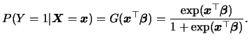
For general aspects on semiparametric regression we refer to the textbooks of Pagan & Ullah (1999), Yatchew (2003), Ruppert et al. (1990). Comprehensive presentations of the generalized linear model can be found in Dobson (2001), McCullagh & Nelder (1989) and Hardin & Hilbe (2001). For a more compact introduction see Müller (2004), Venables & Ripley (2002, Chapter 7) and Gill (2000).

In the following notes, we give some references for topics we consider related to the considered models. References for specific models are listed in the relevant chapters later on.

The transformation model in (5.4) was first introduced in an econometric context by Box & Cox (1964). The discussion was revised many years later by Bickel & Doksum (1981). In a more recent paper, Horowitz (1996) estimates this model by considering a nonparametric transformation.

For a further reference of dimension reduction in nonparametric estimation we mention projection pursuit and sliced inverse regression. The projection pursuit algorithm is introduced and investigated in detail in Friedman & Stuetzle (1981) and Friedman (1987). Sliced inverse regression means the estimation of $Y=m\left( {\boldsymbol{X}}^\top{\boldsymbol{\beta}}_1 ,{\boldsymbol{X}}^\top{\... ...a}}_2,\ldots, {\boldsymbol{X}}^\top{\boldsymbol{\beta}}_k, \varepsilon \right),$ where $\varepsilon$ is the disturbance term and $k$ the unknown dimension of the model. Introduction and theory can be found e.g. in Duan & Li (1991), Li (1991) or Hsing & Carroll (1992).

More sophisticated models like censored or truncated dependent variables, models with endogenous variables or simultaneous equation systems (Maddala, 1983) will not be dealt with in this book. There are two reasons: On one hand the non- or semiparametric estimation of those models is much more complicated and technical than most of what we aim to introduce in this book. Here we only prepare the basics enabling the reader to consider more special problems. On the other hand, most of these estimation problems are rather particular and the treatment of them presupposes good knowledge of the considered problem and its solution in the parametric world. Instead of extending the book considerably by setting out this topic, we limit ourselves here to some more detailed bibliographic notes.

The non- and semiparametric literature on this is mainly separated into two directions, parametric modeling with unknown error distribution or modeling non-/semiparametrically the functional forms. In the second case a principal question is the identifiability of the model.

For an introduction to the problem of truncation, sample selection and limited dependent data, see Heckman (1976) and Heckman (1979). See also the survey of Amemiya (1984). An interesting approach was presented by Ahn & Powell (1993) for parametric censored selection models with nonparametric selection mechanism. This idea has been extended to general pairwise difference estimators for censored and truncated models in Honoré & Powell (1994). A mostly comprehensive survey about parametric and semiparametric methods for parametric models with non- or semiparametric selection bias can be found in Vella (1998). Even though implementation of and theory on these methods is often quite complicated, some of them turned out to perform reasonably well.

The second approach, i.e. relaxing the functional forms of the functions of interest, turned out to be much more complicated. To our knowledge, the first articles on the estimation of triangular simultaneous equation systems have been Newey et al. (1999) and Rodríguez-Póo et al. (1999), from which the former is purely nonparametric, whereas the latter considers nested simultaneous equation systems and needs to specify the error distribution for identifiability reasons. Finally, Lewbel & Linton (2002) found a smart way to identify nonparametric censored and truncated regression functions; however, their estimation procedure is quite technical. Note that so far neither their estimator nor the one of Newey et al. (1999) have been proved to perform well in practice.

EXERCISE 5.1   Assume model (5.6) and consider ${\boldsymbol{X}}$ and $\varepsilon$ to be independent. Show that

$$P(Y=1\vert{\boldsymbol{X}})=E(Y\vert{\boldsymbol{X}})=G_\varepsilon\{v({\boldsymbol{X}})\}$$

where $G_\varepsilon$ denotes the cdf of $\varepsilon$. Explain that (5.7) holds if we do not assume independence of ${\boldsymbol{X}}$ and $\varepsilon$.

EXERCISE 5.2   Recall the paragraph about partial linear models. Why may it be sufficient to include $\beta_1X_1$ in the model when $X_1$ is binary? What would you do if $X_1$ were categorical?

EXERCISE 5.3   Compute ${\mathcal{H}}({\boldsymbol{\beta}})$ and $E{\mathcal{H}}({\boldsymbol{\beta}})$ for the logit and probit models.

EXERCISE 5.4   Verify the canonical link functions for the logit and Poisson model.

EXERCISE 5.5   Recall that in Example 5.6 we have fitted the model

$$E(Y\vert{\boldsymbol{X}})=P(Y=1\vert{\boldsymbol{X}})=G({\boldsymbol{X}}^\top{\boldsymbol{\beta}}),$$

where $G$ is the standard logistic cdf. We motivated this model through the latent-variable model $Y^*={\boldsymbol{X}}^\top{\boldsymbol{\beta}}-\varepsilon$ with $\varepsilon$ having cdf $G$. How does the logit model change if the latent-variable model is multiplied by a factor $c$? What does this imply for the identification of the coefficient vector ${\boldsymbol{\beta}}$?

Summary

$\ast$

The basis for many semiparametric regression models is the generalized linear model (GLM), which is given by

$$E(Y\vert{\boldsymbol{X}}) = G\{ {\boldsymbol{X}}^\top{\boldsymbol{\beta}}\}\,.$$

Here, ${\boldsymbol{\beta}}$ denotes the parameter vector to be estimated and $G$ denotes a known link function. Prominent examples of this type of regression are binary choice models (logit or probit) or count data models (Poisson regression).

$\ast$

The GLM can be generalized in several ways: Considering an unknown smooth link function (instead of $G$) leads to the single index model (SIM). Assuming a nonparametric additive argument of $G$ leads to the generalized additive model (GAM), whereas a combination of additive linear and nonparametric components in the argument of $G$ give a generalized partial linear model (GPLM) or generalized partial linear partial additive model (GAPLM). If there is no link function (or $G$ is the identity function) then we speak of additive models (AM) or partial linear models (PLM) or additive partial linear models (APLM).

$\ast$

The estimation of the GLM is performed through an interactive algorithm. This algorithm, the iteratively reweighted least squares (IRLS) algorithm, applies weighted least squares to the adjusted dependent variable $Z$ in each iteration step:

$${\boldsymbol{\beta}}^{new}= ({\mathbf{X}}^\top {\mathbf{W}}{\mathbf{X}})^{-1} {\mathbf{X}}^\top {\mathbf{W}}{{\boldsymbol{Z}}}$$

This numerical approach needs to be appropriately modified for estimating the semiparametric modifications of the GLM.