8.3 Finite Sample Behavior

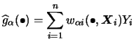
Asymptotic statistical properties are only one part of the story. For the applied researcher knowledge of the finite sample behavior of a method and its robustness are essential. This section is reserved for this topic.

We present and examine now results on the finite sample performance of the competing backfitting and integration approaches. To keep things simple we only use local constant and local linear estimates here. For a more detailed discussion see Sperlich et al. (1999) and Nielsen & Linton (1998). Let us point out again, that

• backfitting always projects the regression problem into the space of additive models,
• marginal integration estimates the marginal impact of a regressor independently of the underlying model.

Thus, both techniques are only comparable in truly additive models. We concentrate here only on the backfitting algorithm as introduced by Hastie & Tibshirani (1990) and the marginal integration as presented in Severance-Lossin & Sperlich (1999).

The following two subsections refer to results for the specific models

$$Y_i = g_a (X_{i1}) + g_b (X_{i2}) +\varepsilon_i ,\quad i=1,\ldots ,n$$

where $a \neq b$ are chosen from $1,\ldots,4$ and

$$\begin{array}{rlcrl} g_{1}(X_{i\bullet})= & 2X_{i\bullet}\,,... ...(X_{i\bullet})= & 0.5\cdot \sin (-1.5X_{i\bullet}). \end{array}$$

Here, the $X_{i\bullet}$ stand for i.i.d. regressor variables that are either uniform on $[-3,3]\times [-3,3]$ distributed or (correlated) bivariate normals with mean 0, variance $1$ and covariance $\rho\in\{0,0.4,0.8\}$. The error terms $\varepsilon_i$ are independently $N(0,0.5)$ distributed. If not mentioned differently, we consider a sample size $n=100$.

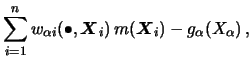
Note that all estimators presented in this section (two-dimensional backfitting and marginal integration estimators) are linear in ${\boldsymbol{Y}}$, i.e. of the form

$$\widehat{g}_{\alpha }(\bullet)=\sum_{i=1}^{n} w_{{\alpha i}}(\bullet,{\boldsymbol{X}}_{i})Y_{i}$$

for some weights $w_{{\alpha }i}(\bullet,{\boldsymbol{X}}_{i\underline{\alpha}})$. Consequently the conditional bias and variance can be calculated by

$$\bias\left\{ \widehat{g}_{\alpha }(\bullet)\vert {\boldsymbol{X}}\right\} = \sum_{i=1}^{n}w_{{\alpha }i}(\bullet,{\boldsymbol{X}}_{i})\,m( {\boldsymbol{X}}_{i}) -g_{\alpha}(X_{\alpha })\,,$$

$$\mathop{\mathit{Var}}\left\{ \widehat{g}_{\alpha }(\bullet)\vert{\boldsymbol{X}}\right\} = \sigma _{\varepsilon }^{2}\sum_{i=1}^{n}w^2_{{\alpha }i}(\bullet,{\boldsymbol{X}}_{i})\,.$$

An analog representation holds for the overall regression estimate $\widehat{m}$. We introduce the notation

$$\mse_t=\mse\{\widehat{g}_\alpha(t)\} =E\left\{\widehat{g}_\alpha(t)-{g}_\alpha(t)\right\}^2$$

for the mean squared error, and

$$\mase=\mase(\widehat{g}_\alpha) =\frac 1n \sum_i \left\{\widehat{g}_\alpha(X_{i\alpha})-{g}_\alpha(X_{i\alpha})\right\}^2$$

for the mean averaged squared error, the density weighted empirical version of the $\mse$. We will also use the analog definitions for $\widehat{m}$.

8.3.1 Bandwidth Choice

As we have already discussed in the first part of this book, the choice of the smoothing parameter is crucial in practice. The integration estimator requires to choose two bandwidths, $h$ for the direction of interest and $\widetilde{h}$ for the nuisance direction. Possible practical approaches are the rule of thumb of Linton & Nielsen (1995) and the plug-in method suggested in Severance-Lossin & Sperlich (1999). Both methods use the MASE-minimizing bandwidth, the former approximating it by means of parametric pre-estimators, the latter one by using nonparametric pre-estimators.

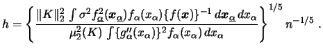
For example, the formula for the MASE-minimizing (and thus asymptotically optimal) bandwidth in the local linear case is given by

$$h = \left\{ \frac{ \Vert K \Vert^2_2 \,\int \sigma^2 f^2_{\underl... ... (x_\alpha ) \}^2 f_\alpha (x_\alpha) \,dx_\alpha } \right\}^{1/5} n^{-1/5} \ .$$ (8.28)

However, simulations in the above cited papers show that in small samples the bandwidths are far away from those obtained by numerical MASE minimization. Note also, that formula (8.28) is not valid for the $\widetilde{h}$. For these bandwidths, the literature recommends undersmoothing. It turns out that this is not essential (in practice). The reason is that the multiplicative term corresponding to $\widetilde{h}$ is often already very small compared to the bias term corresponding to $h$.

In case of backfitting the procedure becomes possible due to the fact that we only consider one-dimensional smoothers. Here, the MASE-minimizing bandwidth is commonly approximated by the MASE-minimizing bandwidth for the corresponding one-dimensional kernel regression case.

EXAMPLE 8.6  
To demonstrate the sensitivity, respectively the robustness of the estimators w.r.t. the choice of the bandwidth we plot MASE and $\mse_{0}$ against $h$ for the two models $m=g_2+g_3$ and $m=g_2+g_4$. We show here only the results for the local linear smoother and the independent designs ${\boldsymbol{X}}\sim U[-3,3]\times U[-3,3]$, ${\boldsymbol{X}}\sim N(0,1)\times N(0,1)$. The MASE and $\mse_{0}$ curves are displayed in Figures 8.9 and 8.10. In all of them, we use thick solid lines for marginal integration and dashed lines for backfitting. $\Box$

Figure 8.9: Performance of MASE (top and third row) and $\mse_{0}$ (second and bottom row) by bandwidth $h$, overall model is $m=g_2+g_3$, the columns represent $g_2$ (left) and $g_3$ (right) under uniform design (upper two rows) and normal design (lower two rows)

Figure 8.10: Performance of MASE (top and third row) and $\mse_{0}$ (second and bottom row) by bandwidth $h$, overall model is $m=g_2+g_4$, the columns represent $g_2$ (left) and $g_3$ (right) under uniform design (upper two rows) and normal design (lower two rows)

Obviously, the backfitting estimator is rather sensitive to the choice of bandwidth. To get small MASE values it is important for the backfitting method to choose the smoothing parameter appropriately. For the integration estimator the results differ depending on the model. This method is nowhere near as sensitive to the choice of bandwidth as the backfitting. Focusing on the $\mse_{0}$ we have similar results as for the MASE but weakened concerning the sensitivity. Here the results differ more depending on the data generating model.

8.3.2 MASE in Finite Samples

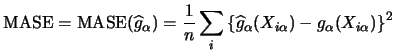
Table 8.1 presents the MASE when using local linear smoothers and the asymptotically optimal bandwidths. To exclude boundary effects each entry of the table consists of two rows: evaluation on the complete data set in the upper row, and evaluation on trimmed data in the lower row. The trimming was implemented by cutting off $5\%$ of the data on each side of the support.

Table 8.1: MASE for backfitting (back) and marginal integration (int) for estimating $g_\alpha$ and $m$, normal designs with different covariances (first row), MASE calculated for the complete (upper row) and the trimmed data (lower row)

covariance		$0.0$	$0.4$	$0.8$	$0.0$	$0.4$	$0.8$	$0.0$	$0.4$	$0.8$	$0.0$	$0.4$	$0.8$
model		$m = g_1 + g_2$			$m = g_1 + g_3$			$m=g_2+g_4$			$m = g_3 + g_4$
	back	0.047	0.041	0.020	0.046	0.028	0.053	0.124	0.135	0.128	0.068	0.081	0.111
		0.038	0.031	0.014	0.037	0.018	0.033	0.107	0.116	0.099	0.046	0.055	0.081
${g}_{a}$	int	0.019	0.030	0.057	0.031	0.075	0.081	0.047	0.048	0.089	0.053	0.049	0.056
		0.013	0.017	0.047	0.024	0.059	0.071	0.022	0.026	0.078	0.026	0.022	0.041
	back	0.083	0.079	0.047	0.073	0.053	0.058	0.112	0.121	0.110	0.051	0.062	0.096
		0.071	0.060	0.024	0.058	0.032	0.028	0.101	0.110	0.091	0.039	0.048	0.075
${g}_{b}$	int	0.090	0.116	0.530	0.137	0.234	0.528	0.048	0.480	1.32	0.057	0.603	2.41
		0.028	0.029	0.205	0.027	0.031	0.149	0.032	0.061	0.151	0.040	0.265	1.02
	back	0.052	0.054	0.049	0.051	0.054	0.057	0.061	0.063	0.068	0.065	0.066	0.064
		0.032	0.031	0.028	0.030	0.029	0.035	0.035	0.035	0.037	0.038	0.037	0.038
${m}$	int	0.115	0.145	0.619	0.175	0.285	0.608	0.118	0.561	1.37	0.085	0.670	2.24
		0.041	0.041	0.252	0.043	0.053	0.194	0.076	0.083	0.189	0.044	0.257	0.681

We see that no estimator is uniformly superior to the others. All results depend more significantly on the design distribution and the underlying model than on the particular estimation procedure. The main conclusion is that backfitting almost always fits the overall regression better whereas the marginal integration often does better for the additive components. Recalling the construction of the procedures this is not surprising, but exactly what one should have expected.

Also not surprisingly, the integration estimator suffers more heavily from boundary effects. For increasing correlation both estimators perform worse, but this effect is especially present for the integration estimator. This is in line with the theory saying that the integration estimator is inefficient for correlated designs, see Linton (1997). Here a bandwidth matrix with appropriate non-zero arguments in the off diagonals can help in case of high correlated regressors, see a corresponding study in Sperlich et al. (1999). They point out that the fit can be improved significantly by using well defined off-diagonal elements in the bandwidth matrices. A similar analysis would be harder to do for the backfitting method as it depends only on one-dimensional smoothers. We remark that internalized marginal integration estimators (Dette et al., 2004) and smoothed backfitting estimators (Mammen et al., 1999; Nielsen & Sperlich, 2002) are much better suited to deal with correlated regressors.

8.3.3 Equivalent Kernel Weights

How do the additive approaches overcome the curse of dimensionality? We compare now the additive estimation method with the bivariate Nadaraya-Watson kernel smoother. We define equivalent kernels as the linear weights $w_i$ used in the estimates for fitting the regression function at a particular point. In the following we take the center point $(0,0)$, which is used in Figures 8.11 to 8.13. All estimators are based on univariate or bivariate Nadaraya-Watson smoothers (in the latter case using a diagonal bandwidth matrix).

Figure 8.11: Equivalent kernels for the bivariate Nadaraya-Watson estimator, normal design with covariance 0 (left) and 0.8 (right)

Figure 8.12: Equivalent kernels for backfitting based on univariate Nadaraya-Watson smoothers, normal design with covariance 0 (left) and 0.8 (right)

Figure 8.13: Equivalent kernels for marginal integration based on bivariate Nadaraya-Watson smoothers, normal design with covariance 0 (left) and 0.8 (right)

Obviously, additive methods (Figures 8.12, 8.13) are characterized by their local panels along the axes instead of being uniformly equal in all directions like the bivariate Nadaraya-Watson (Figure 8.11). Since additive estimators are made up of components that behave like univariate smoothers, they can overcome the curse of dimensionality. The pictures for the additive smoothers look very similar (apart from some negative weights for the backfitting).

Finally, we see clearly how both additive methods run into problems when the correlation between the regressors is increasing. In particular for the marginal integration estimator recall that before we apply the integration over the nuisance directions, we pre-estimate $m$ on all combinations of realizations of $X_1$ and $X_2$. For example, since $X_1,X_2$ are both uniform on $[-1,1]$ it may happen that we have to pre-estimate the regression function at the point $(0.9,-0.9)$. Now imagine that $X_1$ and $X_2$ are positively correlated. In small samples, the pre-estimate for $m(0.9,-0.9)$ is then usually obtained by extrapolation. The insufficient quality of the pre-estimate does then transfer to the final estimate.

EXAMPLE 8.7  
Let us further illustrate the differences and common features of the discussed estimators by means of an explorative real data analysis. We investigate the relation of managerial compensation to firm size and financial performance based on the data used in Grasshoff et al. (1999). Empirical studies show a high pay for firm size sensitivity and a low pay for financial performance sensitivity. These studies use linear, log-linear or semi-log-linear relations.

Consider the empirical model

$$\log (C_{i})=\beta_0 +\beta_1 \log (S_{i})+\beta_2 P_{i}+\varepsilon_{i}$$ (8.29)

for a sample of $n$ firms at different time points $t=1,\ldots ,T$. The explanatory variables are

$C_{i}$

compensation per capita,

$S_{i}$

measure of firm size, here number of employees,

$P_{i}$

measure of financial performance, here the profit to sales ratio (ROS).

The data base for this analysis is drawn from the Kienbaum Vergütungsstudie, containing data about top management compensation of German AGs and the compensation of managing directors (Geschäftsführer) of incorporateds (GmbHs). To measure compensation we use managerial compensation per capita due to the lack of more detailed information. The analysis is based on the following four industry groups.

• group 1 (basic industries)
  consists of companies for chemicals/ pharmaceuticals/ plastics, iron and steel, rubber, mineral oil, non iron ores and cement,
• group 2 (capital goods)
  consists of companies for metal ware /sheet metal, electrical industry, vehicles, precision mechanics and optics, mechanical engineering and ship building,
• group 3 (consumer goods)
  consists of companies for glass/ ceramics and textiles/ clothing,
• group 4 (food, drink, and tobacco )
  consists of companies for breweries, other food, drink and tobacco.

Table 8.2: Parameter estimates for the log-linear model (asterisks indicate significance at the $1\%$ level)

Group	1	2	3	4
# observations	131	148	41	38
constant	4.128$^*$	4.547$^*$	3.776$^*$	4.120$^*$
ROS	1.641	0.959	15.01$^*$	8.377
log(SIZE)	0.258$^*$	0.201$^*$	0.283$^*$	0.249$^*$

Figure 8.14: 3D surface estimates for branch groups 1 to 4 (upper left to lower right)

We first present the results of the parametric analysis for each group, see Table 8.2. The sensitivity parameter for the size variable can be directly interpreted as the size elasticity in each case.

Figure 8.15: Backfitting additive and linear function estimates together with selected data points, branch groups 1 to 4 (from above to below)

We now check for a possible heterogeneous behavior over the groups. A two-dimensional Nadaraya-Watson estimate is shown in Figure 8.14. Considering the plots we realize that the estimated surfaces are similar for the industry groups 1 and 2 (upper row) while the surfaces for the two other groups clearly differ. Further, we see a strong positive relation for compensation to firm size at least in groups 1 and 2, and a weaker one to the performance measure varying over years and groups. Finally, interaction of the regressors -- especially in groups 3 and 4 -- can be recognized.

The backfitting procedure projects the data into the space of additive models. We used for the backfitting estimators univariate local linear kernel smoother with Quartic kernel and bandwidth inflation factors 0.75, 0.5 for group 1 and 2 and 1.25, 1.0 for groups 3 and 4. In the Figure 8.15 we compare the nonparametric (additive) components with the parametric (linear) functions. Over all groups we observe a clear nonlinear impact of ROS. Note, that the low values for significance in the parametric model describe only the linear impact, which here seem to be caused by functional misspecification (or interactions).

Figure 8.16: Marginal integration estimates with $2\sigma$ bands, branch groups 1 to 4 (from above to below)

Finally, in Figure 8.16 we estimate the marginal effects of the regressors using local linear smoothers. The estimated marginal effects are presented together with $2{\sigma }$-bands, where we use for $\sigma$ the variance functions of the estimates. Note that for ROS in group 1 the ranges are slightly different as in Figure 8.15.

Generally, the results are consistent with the findings above. The nonlinear effects in the impact of ROS are stronger, especially in groups 1 and 2. Since the abovementioned bumps in the firm size do not exist here, we can conclude that indeed interaction effects are responsible for this. The backfitting results differ substantially from the estimated marginal effects in group 3 and 4 what again underlines the presence of interaction effects.

To summarize, we conclude that the separation into groups is useful, but groups 1 and 2 respectively 3 and 4 seem to behave similarly. The assumption of additivity seems to be violated for groups 3 and 4. Furthermore, the nonparametric estimates yield different results due to nonlinear effects and interaction, so that parametric elasticities underestimate the true elasticity in our example. $\Box$

Additive models were first considered for economics and econometrics by Leontief (1947a,b). Intensive discussion of their application to economics can be found in Deaton & Muellbauer (1980) and Fuss et al. (1978). Wecker & Ansley (1983) introduced especially the backfitting method in economics.

The development of the backfitting procedure has a long history. The procedure goes back to algorithms of Friedman & Stuetzle (1982) and Breiman & Friedman (1985). We also refer to Buja et al. (1989) and the references therein. Asymptotic theory for backfitting has been studied first by Opsomer & Ruppert (1997), and later on (under more general conditions) in the above mentioned paper of Mammen et al. (1999).

The marginal integration estimator was first presented by Tjøstheim & Auestad (1994a) and Linton & Nielsen (1995), the idea can also be found in Newey (1994) or Boularan et al. (1994) for estimating growth curves. Hengartner et al. (1999) introduce modifications leading to computational efficiency. Masry & Tjøstheim (1997); Masry & Tjøstheim (1995) use marginal integration and prove its consistency in the context of time series analysis. Dalelane (1999) and Achmus (2000) prove consistency of bootstrap methods for marginal integration. Linton (1997) combines marginal integration and a one step backfitting iteration to obtain an estimator that is both efficient and easy to analyze.

Interaction models have been considered in different papers. Stone et al. (1997) and Andrews & Whang (1990) developed estimators for interaction terms of any order by polynomial splines. Spline estimators have also been used by Wahba (1990). For series estimation we refer in particular to Newey (1995) and the references therein. Härdle et al. (2001) use wavelets to test for additive models. Testing additivity is a field with a growing amount of literature, such as Chen et al. (1995), Eubank et al. (1995) and Gozalo & Linton (2001).

A comprehensive resource for additive modeling is is the textbook by Hastie & Tibshirani (1990) who focus on the backfitting approach. Further references are Sperlich (1998) and Ruppert et al. (1990).

EXERCISE 8.1   Assume that the regressor variable $X_1$ is independent from $X_2,\ldots ,X_d$. How does this change the marginal integration estimator now? Interpret this change.

EXERCISE 8.2   When using the local linear smoother for backfitting, what would be the optimal bandwidth for estimating linear functions?

EXERCISE 8.3   Give at least two methods of constructing confidence intervals for the component function estimates. Consider both the backfitting and the marginal integration method. Discuss also approaches for the construction of confidence bands.

EXERCISE 8.4   We mentioned that backfitting procedures could be implemented using any one-dimensional smoother. Discuss the analog issue for the marginal integration method.

EXERCISE 8.5   Assume we have been given a regression problem with five explanatory variables and a response $Y$. Our aim is to predict $Y$ but we are not really interested in the particular impact of each input. Although we do not know whether the model is additive, the curse of dimensionality forces us to think about dimension reduction and we decide upon an additive approach. Which estimation procedure will you recommend?

EXERCISE 8.6   Recall Subsection 8.3.3. Does the underlying model matter for construction or interpretation of Figures 8.11 to 8.13? Justify your answer.

EXERCISE 8.7   Recall Subsection 8.2.3 where we considered models of the form

$$m({\boldsymbol{X}})=c+\sum_{\alpha = 1}^d g_\alpha (X_\alpha )+\sum_{1\leq \alpha < j \leq d} g_{\alpha j}(X_\alpha ,X_j) \,,$$

i.e. additive models with pairwise interaction terms. We introduced identification and estimation in the context of marginal integration. Discuss the problem now for the backfitting method. In what sense does the main difference between backfitting and marginal integration kick in here?

EXERCISE 8.8   Again, recall Subsection 8.2.3, but now extend the model to

$$m({\boldsymbol{X}})=c+\sum_{\alpha = 1}^d g_\alpha (X_\alpha )+\s... ...X_j) + \sum_{1\leq \alpha < j <k \leq d} g_{\alpha jk} (X_\alpha ,X_j, X_k)\,.$$

How could this model be identified and estimated?

EXERCISE 8.9   Discuss the possibility of modeling some of the component functions $g_\alpha$ parametrically. What would be the advantage of doing so?

EXERCISE 8.10   Assume we have applied backfitting and marginal integration in a high dimensional regression problem. It turns out that we obtain very different estimates for the additive component functions. Discuss the reasons which can cause this effect.

EXERCISE 8.11   How should the formula for the MASE-minimizing bandwidth (8.28) be modified if we consider the local constant case?

Summary

$\ast$

Additive models are of the form

$$E( Y \vert{\boldsymbol{X}}) = m({\boldsymbol{X}})=c+\sum_{\alpha =1}^d g_\alpha (X_\alpha ).$$

In estimation they can combine flexible nonparametric modeling of many variables with statistical precision that is typical of just one explanatory variable, i.e. they circumvent the curse of dimensionality.

$\ast$

In practice, there exist mainly two estimation procedures, backfitting and marginal integration. If the real model is additive, then there are many similarities in terms of what they do to the data. Otherwise their behavior and interpretation are rather different.

$\ast$

The backfitting estimator is an iterative procedure of the kind:

$$\widehat{{\boldsymbol{g}}}_\alpha ^{(l)}={\mathbf{S}}_\alpha \lef... ...q \alpha }\widehat{{\boldsymbol{g}}}_j ^{(l-1)}\right\} ,\quad l=1,2,3, \ldots$$

until some prespecified tolerance is reached. This is a successive one-dimensional regression of the partial residuals on the corresponding $X_\alpha$.

$\ast$

Usually backfitting fits the regression better than the integration estimator. But it pays for a low MSE (or MASE) for the regression with high MSE (MASE respectively) in the additive function estimation. Furthermore, it is rather sensitive against the bandwidth choice. Also, an increase in the correlation $\rho$ of the design leads to a worse estimate.

$\ast$

The marginal integration estimator is based on the idea that

$$E_{{\boldsymbol{X}}_{\underline{\alpha}}} \{ m ( X_\alpha , {\boldsymbol{X}}_{\underline{\alpha}} \} = c+g_\alpha (X_\alpha ).$$

Replacing $m$ by a pre-estimator and the expectation by averaging defines a consistent estimate.

$\ast$

Marginal integration suffers more from sparseness of observations than the backfitting estimator does. So for example the boundary effects are worse for the integration estimator. In the center of the support of ${\boldsymbol{X}}$ this estimator mostly has lower MASE for the estimators of the additive component functions. An increasing covariance of the explanatory variables affects the MASE strongly in a negative sense. Regarding the bandwidth this estimator seems to be quite robust.

$\ast$

If the real model is not additive, the integration estimator is estimating the marginals by integrating out the directions of no interest. In contrast, the backfitting estimator is looking in the space of additive models for the best fit of the response $Y$ on ${\boldsymbol{X}}$.