1.9 Exercises

EXERCISE 1.3 Assume that the data are normally distributed

. What percentage of the data do you expect to lie outside the outside bars?

EXERCISE 1.4 What percentage of the data do you expect to lie outside the outside bars if we assume that the data are normally distributed $N(0,\sigma^2)$ with unknown variance $\sigma^2$ ?

EXERCISE 1.5 How would the five-number summary of the 15 largest U.S. cities differ from that of the 50 largest U.S. cities? How would the five-number summary of 15 observations of

-distributed data differ from that of 50 observations from the same distribution?

EXERCISE 1.7 Suppose we have

observations of $X\sim N(0,1)$ and another

observations of $Y\sim N(2,1)$ . What would the

Flury faces look like if you had defined as face elements the face line and the darkness of hair? Do you expect any similar faces? How many faces do you think should look like observations of

even though they are

observations?

EXERCISE 1.8 Draw a histogram for the mileage variable of the car data (Table B.3). Do the same for the three groups (U.S., Japan, Europe). Do you obtain a similar conclusion as in the parallel boxplot on Figure 1.3 for these data?

EXERCISE 1.9 Use some bandwidth selection criterion to calculate the optimally chosen bandwidth

for the diagonal variable of the bank notes. Would it be better to have one bandwidth for the two groups?

EXERCISE 1.10 In Figure 1.9 the densities overlap in the region of diagonal $\approx 140.4$ . We partially observed this in the boxplot of Figure 1.4. Our aim is to separate the two groups. Will we be able to do this effectively on the basis of this diagonal variable alone?

EXERCISE 1.12 How would you identify discrete variables (variables with only a limited number of possible outcomes) on a parallel coordinates plot?

EXERCISE 1.13 True or false: the height of the bars of a histogram are equal to the relative frequency with which observations fall into the respective bins.

EXERCISE 1.14 True or false: kernel density estimates must always take on a value between 0 and 1. (Hint: Which quantity connected with the density function has to be equal to 1? Does this property imply that the density function has to always be less than 1?)

EXERCISE 1.15 Let the following data set represent the heights of 13 students taking the Applied Multivariate Statistical Analysis course:

$\begin{displaymath}1.72,1.83,1.74,1.79,1.94,1.81,1.66,1.60,1.78,1.77,1.85,1.70,1.76.\end{displaymath}$

Find the corresponding five-number summary.
Construct the boxplot.
Draw a histogram for this data set.

Contributed by Peder Egemen Baykan.

EXERCISE 1.16 Describe the unemployment data (see Table B.19) that contain unemployment rates of all German Federal States using various descriptive techniques.

Contributed by Susanne Böhme.

EXERCISE 1.17 Using yearly population data (see B.20), generate

a boxplot (choose one of variables)
an Andrew's Curve (choose ten data points)
a scatterplot
a histogram (choose one of the variables)

What do these graphs tell you about the data and their structure?

Contributed by Susanne Böhme.

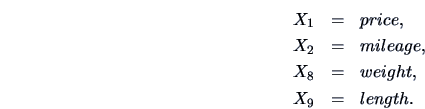
EXERCISE 1.18 Make a draftman plot for the car data with the variables

$\begin{eqnarray*} X_{1} & = & price, \\ X_{2} & = & mileage, \\ X_{8} & = & weight, \\ X_{9} & = & length. \end{eqnarray*}$

Move the brush into the region of heavy cars. What can you say about price, mileage and length? Move the brush onto high fuel economy. Mark the Japanese, European and U.S. American cars. You should find the same condition as in boxplot Figure 1.3.

EXERCISE 1.19 What is the form of a scatterplot of two independent random variables $X_{1}$ and $X_{2}$ with standard Normal distribution?

EXERCISE 1.20 Rotate a three-dimensional standard normal point cloud in 3D space. Does it ``almost look the same from all sides''? Can you explain why or why not?