1.3 Kernel Densities
The major difficulties of histogram estimation may be summarized
in four critiques:
- determination of the binwidth
 , which controls the shape of the histogram,
- choice of the bin origin
 , which also influences to some extent the shape,
- loss of information since observations are replaced by the central point of the interval in which they fall,
- the underlying density function is often assumed to be smooth, but the histogram is not smooth.
Rosenblatt (1956), Whittle (1958), and Parzen (1962) developed an
approach which avoids the last three difficulties.
First, a smooth kernel function rather than a box is used as the basic
building block. Second, the smooth function is centered directly over
each observation.
Let us study this refinement by supposing
that  is the center value of a bin.
The histogram can in fact be rewritten as
is the center value of a bin.
The histogram can in fact be rewritten as
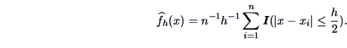 |
(1.8) |
If we define
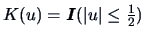 , then (1.8)
changes to
, then (1.8)
changes to
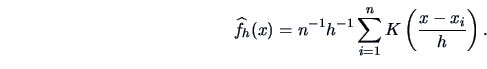 |
(1.9) |
This is the general form of the kernel estimator.
Allowing smoother kernel functions like the quartic kernel,
and computing not only at bin centers gives us the kernel density
estimator. Kernel estimators can also be derived via weighted averaging of
rounded points (WARPing) or by averaging histograms with different
origins, see Scott (1985).
Table 1.3 introduces some commonly used kernels.
Table 1.3:
Kernel functions.
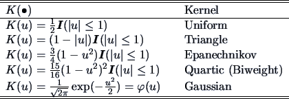 |
Figure:
Densities of the diagonals of genuine and counterfeit bank notes.
Automatic density estimates.
 MVAdenbank.xpl
|
|
Figure:
Contours of the density of  and
and  of
genuine and counterfeit bank notes.
MVAcontbank2.xpl
of
genuine and counterfeit bank notes.
MVAcontbank2.xpl
|
|
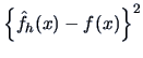
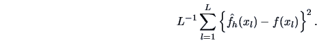
Different kernels generate different shapes of the estimated density.
The most important parameter is the so-called bandwidth , and
can be optimized, for example, by cross-validation;
see Härdle (1991) for details. The cross-validation method
minimizes the integrated squared error.
This measure of discrepancy is based on the squared differences
 . Averaging these squared deviations
over a grid of points
. Averaging these squared deviations
over a grid of points
 leads to
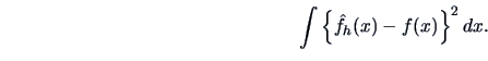
Asymptotically, if this grid size tends to zero, we obtain the
integrated squared error:
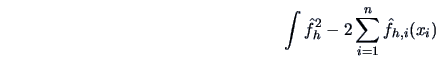
In practice, it turns out that the method consists of selecting
a bandwidth that minimizes the cross-validation function
where  is the density estimate obtained by using all datapoints except for
the
is the density estimate obtained by using all datapoints except for
the  -th observation. Both terms in the above function involve double
sums. Computation may therefore be slow.
There are many other density bandwidth selection methods.
Probably the fastest way to calculate this is to refer to some
reasonable reference distribution. The idea of using the Normal distribution
as a reference, for example, goes back to Silverman (1986).
The resulting choice of is called the rule of thumb.
-th observation. Both terms in the above function involve double
sums. Computation may therefore be slow.
There are many other density bandwidth selection methods.
Probably the fastest way to calculate this is to refer to some
reasonable reference distribution. The idea of using the Normal distribution
as a reference, for example, goes back to Silverman (1986).
The resulting choice of is called the rule of thumb.
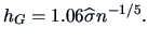
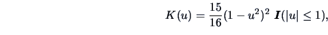
For the Gaussian kernel from Table 1.3
and a Normal reference distribution, the rule of thumb is to choose
 |
(1.10) |
where
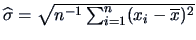 denotes the sample standard deviation.
This choice of
denotes the sample standard deviation.
This choice of  optimizes the integrated squared distance
between the estimator and the true
density. For the quartic kernel, we need to transform (1.10).
The modified rule of thumb is:
optimizes the integrated squared distance
between the estimator and the true
density. For the quartic kernel, we need to transform (1.10).
The modified rule of thumb is:
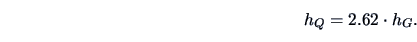 |
(1.11) |
Figure 1.9 shows the automatic density estimates
for the diagonals of the counterfeit and genuine bank notes.
The density on the left is the density corresponding
to the diagonal of the counterfeit data.
The separation is clearly visible, but there is also an overlap.
The problem of distinguishing between the counterfeit and
genuine bank notes is not solved by just looking at the diagonals of
the notes! The question arises whether a better separation
could be achieved using
not only the diagonals but one or two more variables of the data set.
The estimation of higher dimensional densities is analogous to that
of one-dimensional. We show a two dimensional density
estimate for and  in Figure 1.10.
The contour lines indicate the height of the density. One sees two separate
distributions in this higher dimensional space, but they still
overlap to some extent.
in Figure 1.10.
The contour lines indicate the height of the density. One sees two separate
distributions in this higher dimensional space, but they still
overlap to some extent.
Figure:
Contours of the density of
 of
genuine and counterfeit bank notes.
MVAcontbank3.xpl
of
genuine and counterfeit bank notes.
MVAcontbank3.xpl
|
|
We can add one more dimension and give
a graphical representation of a three dimensional
density estimate, or more precisely an estimate of the joint distribution of
, and . Figure 1.11
shows the contour areas at 3 different levels of the density:
 (light grey),
  (grey), and
  (black) of this three
dimensional density estimate. One can clearly recognize two
``ellipsoids'' (at each level), but as before, they overlap.
In Chapter 12 we will learn how to separate the two ellipsoids and
how to develop a discrimination rule to distinguish between these data points.
(black) of this three
dimensional density estimate. One can clearly recognize two
``ellipsoids'' (at each level), but as before, they overlap.
In Chapter 12 we will learn how to separate the two ellipsoids and
how to develop a discrimination rule to distinguish between these data points.
Summary

- Kernel densities estimate distribution densities by the
kernel method.
- The bandwidth determines the degree of smoothness of the
estimate
 .
.
- Kernel densities are smooth functions and they can graphically
represent distributions (up to 3 dimensions).
- A simple (but not necessarily correct) way to find a good bandwidth
is to compute the rule of thumb bandwidth
 This bandwidth is to be used only in combination with a
Gaussian kernel
This bandwidth is to be used only in combination with a
Gaussian kernel  .
.
- Kernel density estimates are a good descriptive tool for seeing
modes, location, skewness, tails, asymmetry, etc.
![\includegraphics[width=1\defpicwidth]{denbank.ps}](mvahtmlimg142.gif)
![\includegraphics[width=1\defpicwidth]{contbank2.ps}](mvahtmlimg143.gif)
![\includegraphics[width=1.1\defpicwidth]{contbank3.ps}](mvahtmlimg155.gif)