2.2 Spectral Decompositions
The computation of eigenvalues and eigenvectors is an important issue in
the analysis of matrices.
The spectral decomposition or Jordan decomposition links the structure of
a matrix to the eigenvalues and the eigenvectors.
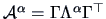
THEOREM 2.1 (Jordan Decomposition)
Each symmetric matrix

can be written as
 |
(2.18) |
where
and where
is an orthogonal matrix consisting of the eigenvectors

of

.
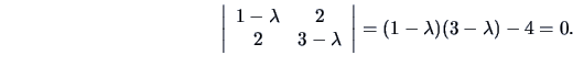
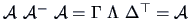
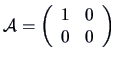
EXAMPLE 2.4
Suppose that

.
The eigenvalues are found by solving
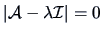
.
This is equivalent to
Hence, the eigenvalues are

and

.
The eigenvectors are
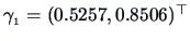
and
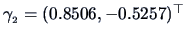
.
They are orthogonal since

.
Using spectral decomposition, we can define powers of a matrix
 . Suppose
  is a symmetric matrix.
Then by Theorem 2.1
is a symmetric matrix.
Then by Theorem 2.1
and we define for some

 |
(2.19) |
where
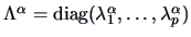 .
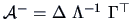
In particular, we can easily calculate the inverse of the matrix
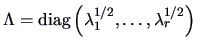
. Suppose that the eigenvalues of are positive. Then
with
.
In particular, we can easily calculate the inverse of the matrix
. Suppose that the eigenvalues of are positive. Then
with  , we obtain the inverse of from
 |
(2.20) |
Another interesting decomposition which is later used is given in
the following theorem.
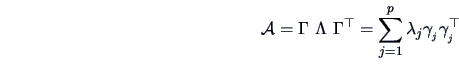
THEOREM 2.2 (Singular Value Decomposition
)
Each matrix

with rank

can be decomposed as
where

and

. Both

and

are column orthonormal, i.e.,
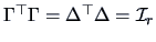
and
,

.
The values

are the non-zero eigenvalues of the
matrices

and

.
and
consist of the corresponding
eigenvectors of
these matrices.
This is obviously a generalization of Theorem 2.1 (Jordan
decomposition). With Theorem 2.2, we can find a  -inverse
 of . Indeed, define
 . Then
 . Note that the -inverse is
not unique.
. Note that the -inverse is
not unique.
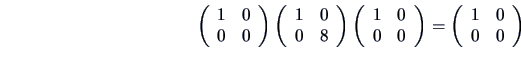
EXAMPLE 2.5
In Example
2.2, we showed that the generalized inverse
of
is
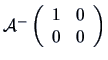
. The following also holds
which means that the matrix

is also a generalized inverse of
.
Summary

- The Jordan decomposition gives a representation of a
symmetric matrix in terms of eigenvalues and eigenvectors.
- The eigenvectors belonging to the largest eigenvalues
indicate the ``main direction'' of the data.
- The Jordan decomposition allows one to easily compute the power
of a symmetric matrix :
 .
.
- The singular value decomposition (SVD) is a generalization
of the Jordan decomposition to non-quadratic matrices.