In multivariate statistics, we observe the values of a multivariate random
variable ![]() and obtain a sample
and obtain a sample
![]() ,
as described in Chapter 3.
Under random sampling, these observations are considered to be realizations of
a sequence of i.i.d. random variables
,
as described in Chapter 3.
Under random sampling, these observations are considered to be realizations of
a sequence of i.i.d. random variables
![]() , where each
, where each ![]() is a
is a
![]() -variate random variable which replicates the parent or population random variable
-variate random variable which replicates the parent or population random variable ![]() . Some notational
confusion is hard to avoid:
. Some notational
confusion is hard to avoid:
![]() is not the
is not the ![]() th component of
th component of ![]() , but rather the
, but rather the ![]() th
replicate of the
th
replicate of the ![]() -variate random variable
-variate random variable ![]() which provides the
which provides the ![]() th
observation
th
observation ![]() of our sample.
of our sample.
For a given random sample
![]() ,
the idea of statistical inference is to analyze the properties of the
population variable
,
the idea of statistical inference is to analyze the properties of the
population variable ![]() . This is typically done by analyzing some
characteristic
. This is typically done by analyzing some
characteristic ![]() of its distribution, like the mean, covariance
matrix, etc. Statistical inference in a
multivariate setup is considered in more detail
in Chapters 6 and 7.
of its distribution, like the mean, covariance
matrix, etc. Statistical inference in a
multivariate setup is considered in more detail
in Chapters 6 and 7.
Inference can often
be performed using some observable function of the sample
![]() ,
i.e., a statistics.
Examples of such statistics were given in Chapter 3:
the sample mean
,
i.e., a statistics.
Examples of such statistics were given in Chapter 3:
the sample mean ![]() ,
the sample covariance matrix
,
the sample covariance matrix ![]() .
To get an idea of the relationship between a statistics and the corresponding
population characteristic, one has to derive the sampling distribution of the
statistic.
The next example gives some insight into the relation of
.
To get an idea of the relationship between a statistics and the corresponding
population characteristic, one has to derive the sampling distribution of the
statistic.
The next example gives some insight into the relation of
![]() to
to ![]() .
.
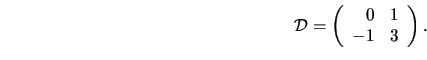
![\begin{displaymath}\begin{array}{lcl}
E(\bar{x}) &=& \frac{1}{n}\sum\limits_{i=1...
...p}\right)\right\}\\ [3mm]
&=& \frac{n-1}{n}\Sigma.
\end{array}\end{displaymath}](mvahtmlimg1456.gif)
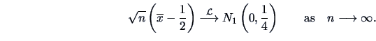
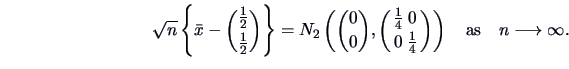
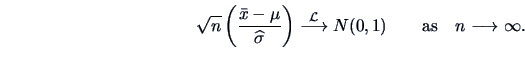
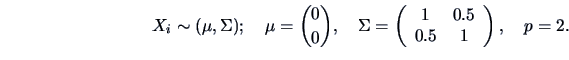
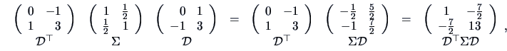
Statistical inference often requires more than just the mean and/or the variance of a statistic. We need the sampling distribution of the statistics to derive confidence intervals or to define rejection regions in hypothesis testing for a given significance level. Theorem 4.9 gives the distribution of the sample mean for a multinormal population.
PROOF:
![]() is a linear combination of independent normal
variables, so it has a normal distribution (see chapter 5). The mean and the
covariance matrix were given in the preceding example.
is a linear combination of independent normal
variables, so it has a normal distribution (see chapter 5). The mean and the
covariance matrix were given in the preceding example.
![]()
With multivariate statistics, the sampling distributions of the
statistics are often
more difficult to derive than in the preceding Theorem.
In addition they might be so
complicated that approximations have to be used. These approximations are
provided by limit theorems. Since they are based on asymptotic limits, the
approximations are only valid when
the sample size is large enough. In spite of this restriction, they make
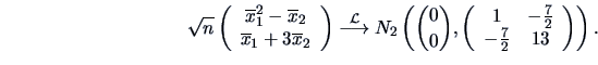
complicated situations rather simple. The following central limit theorem
shows that even if the parent distribution is not normal, when the sample size
![]() is large, the sample mean
is large, the sample mean ![]() has an approximate normal distribution.
has an approximate normal distribution.
The symbol ``
![]() '' denotes convergence
in distribution which means that the distribution function of the random
vector
'' denotes convergence
in distribution which means that the distribution function of the random
vector
![]() converges to the distribution function of
converges to the distribution function of
![]() .
.
![\includegraphics[width=0.6\defepswidth]{cltberna.ps}](mvahtmlimg1473.gif)
![\includegraphics[width=0.6\defepswidth]{cltbernb.ps}](mvahtmlimg1474.gif)
|
The asymptotic normal distribution is often used to construct
confidence intervals for the unknown parameters. A confidence interval
at the level
![]() , is an interval that
covers the true parameter with probability
, is an interval that
covers the true parameter with probability ![]() :
:
where ![]() denotes the (unknown) parameter and
denotes the (unknown) parameter and
![]() and
and
![]() are
the lower and upper confidence
bounds respectively.
are
the lower and upper confidence
bounds respectively.

![\begin{displaymath}\left[\bar{x}-\frac{\sigma}{\sqrt{n}}\, u_{1-\alpha/2},\,
\bar{x}+\frac{\sigma}{\sqrt{n}}\, u_{1-\alpha/2}\right]\end{displaymath}](mvahtmlimg1493.gif)
But what can we do if we do not know the variance ![]() ? The following
corollary gives the answer.
? The following
corollary gives the answer.
![\begin{displaymath}C_{1-\alpha} = \left[\bar{x}-\frac{\widehat{\sigma}}{\sqrt{n}...
...r{x}+\frac{\widehat{\sigma}}{\sqrt{n}}\, u_{1-\alpha/2}\right].\end{displaymath}](mvahtmlimg1500.gif)
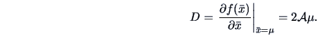
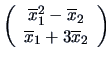
Often in practical problems, one is interested in a function of parameters
for which one has an asymptotically normal statistic. Suppose for instance
that we are interested in a cost function depending on the mean ![]() of the
process:
of the
process:
![]() where
where ![]() is given.
To estimate
is given.
To estimate ![]() we use the asymptotically normal statistic
we use the asymptotically normal statistic ![]() .
The question is: how does
.
The question is: how does ![]() behave? More generally,
what happens to a statistic
behave? More generally,
what happens to a statistic ![]() that is asymptotically normal when we
transform it by a function
that is asymptotically normal when we
transform it by a function ![]() ?
The answer is given by the following theorem.
?
The answer is given by the following theorem.
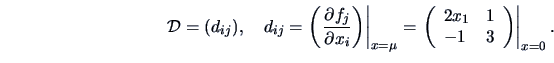
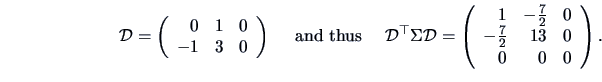
| (4.56) |
 . According
to Theorem 4.11 we have to consider
. According
to Theorem 4.11 we have to consider
![\includegraphics[width=0.6\defepswidth]{cltbern2.ps}](mvahtmlimg1480.gif)
![\includegraphics[width=0.6\defepswidth]{cltbern3.ps}](mvahtmlimg1481.gif)