3.3 Summary Statistics
This section focuses on the representation of basic summary statistics
(means, covariances and correlations)
in matrix notation, since we often apply
linear transformations to data. The matrix notation allows us to derive
instantaneously the corresponding characteristics of the transformed
variables. The Mahalanobis transformation is a prominent example of such
linear transformations.
Assume that we have observed  realizations of a
  -dimensional random
variable; we have a data matrix
-dimensional random
variable; we have a data matrix
 :
:
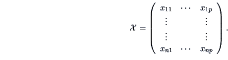 |
(3.16) |
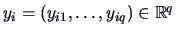
The rows
 denote the
  -th
observation of a -dimensional random variable
-th
observation of a -dimensional random variable
 .
.
The statistics that were briefly introduced in Section 3.1
and 3.2 can be rewritten in
matrix form as follows.
The ``center of gravity'' of the observations in  is given by
the vector
is given by
the vector  of the means
 of the variables:
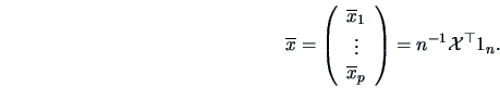 |
(3.17) |
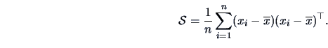
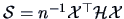
The dispersion of the observations can be characterized by the
covariance matrix of the variables. The empirical covariances
defined in (3.2) and (3.3)
are the elements of the following matrix:
 |
(3.18) |
Note that this matrix is equivalently defined by
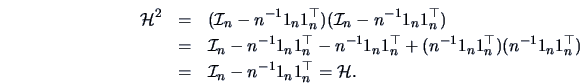
The covariance formula (3.18) can be rewritten as
 with the centering matrix
 |
(3.19) |
Note that the centering matrix is symmetric and idempotent. Indeed,
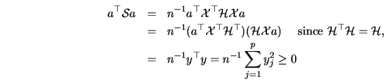
As a consequence  is positive semidefinite, i.e.
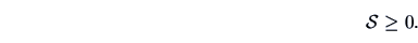 |
(3.20) |
Indeed for all
 ,
,
for
 . It is well known from the one-dimensional
case that
. It is well known from the one-dimensional
case that
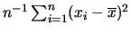 as an estimate of the
variance exhibits a bias of the order
as an estimate of the
variance exhibits a bias of the order  (Breiman; 1973).
In the multidimensional case,
(Breiman; 1973).
In the multidimensional case,
 is an unbiased estimate of the true covariance. (This will be shown in Example
4.15.)
is an unbiased estimate of the true covariance. (This will be shown in Example
4.15.)
The sample correlation coefficient between the -th and  -th variables is
 , see (3.8).
If
, see (3.8).
If
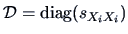 , then the correlation matrix is
 |
(3.21) |
where
 is a diagonal matrix with elements
 on its main diagonal.
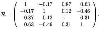
EXAMPLE 3.8
The empirical covariances are calculated for the pullover data set.
The vector of the means of the four variables in the dataset is
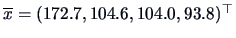 .
.
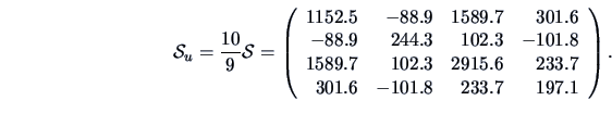
The sample covariance matrix is
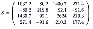
The unbiased estimate of the variance ( =10)
is equal to
The sample correlation matrix is
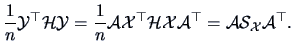
Linear Transformation
In many practical applications we need to study linear transformations of the
original data. This motivates the question of how to calculate
summary statistics after such linear transformations.
Let  be a (
 ) matrix and consider the transformed
data matrix
) matrix and consider the transformed
data matrix
 |
(3.22) |
The row
 can be viewed as the -th
observation of a
can be viewed as the -th
observation of a  -dimensional random variable
  .
In fact we have
.
In fact we have
 .
We immediately obtain the mean and the empirical covariance of the
variables (columns) forming the data matrix
.
We immediately obtain the mean and the empirical covariance of the
variables (columns) forming the data matrix  :
:
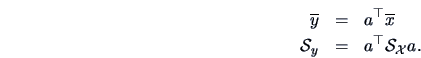
Note that if the linear transformation is
nonhomogeneous, i.e.,
only (3.23) changes:
 .
The formula (3.23) and (3.24) are useful in the
particular case of
.
The formula (3.23) and (3.24) are useful in the
particular case of  , i.e.,
 :
:
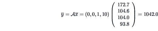
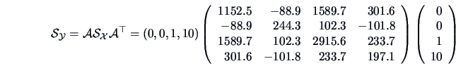
EXAMPLE 3.9
Suppose that

is the pullover data set. The manager wants to
compute his mean expenses for advertisement (

)
and sales assistant (

).
Suppose that the sales assistant charges an hourly wage of 10 EUR. Then the
shop manager calculates the expenses  as
as
 . Formula (3.22) says that this
is equivalent to defining the matrix
. Formula (3.22) says that this
is equivalent to defining the matrix
 as:
as:
Using formulas (
3.23) and (
3.24), it is now computationally
very easy to obtain
the sample mean

and the sample variance

of the
overall expenses:
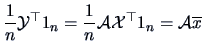
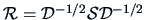
Mahalanobis Transformation
A special case of this linear transformation is
 |
(3.25) |
Note that for the transformed data matrix
 ,
,
 |
(3.26) |
So the Mahalanobis transformation eliminates the correlation between the
variables and standardizes the variance of each variable.
If we apply (3.24) using
 , we obtain
the identity covariance matrix as indicated in (3.26).
, we obtain
the identity covariance matrix as indicated in (3.26).
Summary

-
The center of gravity of a data matrix is given by its mean vector
 .
.
-
The dispersion of the observations in a data matrix is given by the
empirical covariance matrix
.
-
The empirical correlation matrix is given by
 .
.
-
A linear transformation
 of a data matrix
has mean
of a data matrix
has mean
 and empirical covariance
 .
.
-
The Mahalanobis transformation is a linear transformation
 which gives a standardized,
uncorrelated data matrix
which gives a standardized,
uncorrelated data matrix  .
.