3.1 Covariance

Covariance is a measure of dependency between random variables. Given two (random) variables $X$ and $Y$ the (theoretical) covariance is defined by:

$$\sigma _{XY} = \Cov(X,Y)=E(XY)-(EX)(EY).$$ (3.1)

The precise definition of expected values is given in Chapter 4. If $X$ and $Y$ are independent of each other, the covariance $\mathop{\mathit{Cov}}(X,Y)$ is necessarily equal to zero, see Theorem 3.1. The converse is not true. The covariance of $X$ with itself is the variance:

$$\sigma _{XX}=\mathop{\mathit{Var}}(X)=\mathop{\mathit{Cov}}(X,X).$$

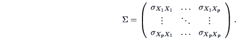
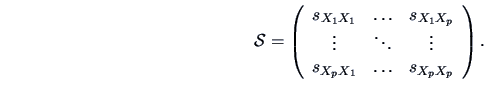
If the variable $X$ is $p$-dimensional multivariate, e.g., $X = \left( \begin{array}{c} X_{1} \\ \vdots \\ X_{p} \end{array} \right)$, then the theoretical covariances among all the elements are put into matrix form, i.e., the covariance matrix:

$$%%\vbox{ \quad {{\Sigma }} = \left ( {\begin{array}{ccc} \sig... ...igma_{X_pX_1}& \ldots & \sigma_{X_pX_p} \end{array}} \right ).$$

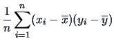
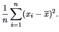
Properties of covariance matrices will be detailed in Chapter 4. Empirical versions of these quantities are:

$$s_{XY} = \frac{1 }{n }\sum ^n_{i=1}(x_i-\overline x)(y_i-\overline y)$$ (3.2)

$$s_{XX} = \frac{1 }{n }\sum ^n_{i=1}(x_i-\overline x)^2.$$ (3.3)

For small $n$, say $n \leq 20$, we should replace the factor $\frac{1}{n}$ in (3.2) and (3.3) by $\frac{1}{n-1}$ in order to correct for a small bias. For a $p$-dimensional random variable, one obtains the empirical covariance matrix (see Section 3.3 for properties and details)

$$%%\vbox{ \quad {\data{S}} = \left ( {\begin{array}{ccc} s_{X_... ...ts \\ s_{X_pX_1}& \ldots & s_{X_pX_p} \end{array}} \right ).$$

For a scatterplot of two variables the covariances measure ``how close the scatter is to a line''. Mathematical details follow but it should already be understood here that in this sense covariance measures only ``linear dependence''.

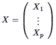
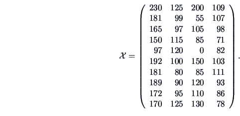
EXAMPLE 3.1   If ${\data{X}}$ is the entire bank data set, one obtains the covariance matrix $\data{S}$ as indicated below:

$${\data{S}} = \left ( {\begin{array}{rrrrrr}\ 0.14&0.03&0.02&... ...4\\ 0.08&-0.21&-0.24&-1.03&-0.54&1.32 \end{array}} \right) .$$ (3.4)

The empirical covariance between $X_4$ and $X_5$, i.e., $s_{X_{4}X_{5}}$, is found in row 4 and column 5. The value is $s_{X_{4}X_{5}}$ = 0.16. Is it obvious that this value is positive? In Exercise 3.1 we will discuss this question further.

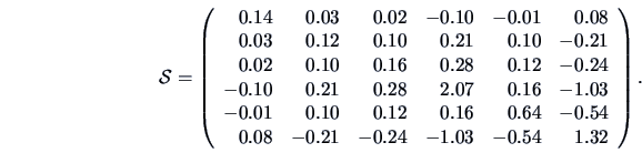
If $\data{X}_{f}$ denotes the counterfeit bank notes, we obtain:

$${\data{S}_{f}} = \left ( {\begin{array}{rrrrrr}\ 0.123& 0.0... ...005& 0.034& 0.236& -0.022& 0.308\\ \end{array}} \right)\cdot$$ (3.5)

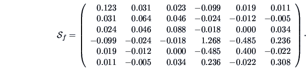
For the genuine, $\data{X}_{g}$, we have:

$${\data{S}_{g}} = \left ( {\begin{array}{rrrrrr}\ 0.149& 0.05... ...3& -0.024& -0.000& -0.074& 0.198\\ \end{array}} \right)\cdot$$ (3.6)

Note that the covariance between $X_4$ (distance of the frame to the lower border) and $X_5$ (distance of the frame to the upper border) is negative in both (3.5) and (3.6)! Why would this happen? In Exercise 3.2 we will discuss this question in more detail.

At first sight, the matrices ${\data{S}_{f}}$ and ${\data{S}_{g}}$ look different, but they create almost the same scatterplots (see the discussion in Section 1.4). Similarly, the common principal component analysis in Chapter 9 suggests a joint analysis of the covariance structure as in Flury and Riedwyl (1988).

Figure 3.1: Scatterplot of variables $X_4$ vs. $X_5$ of the entire bank data set. MVAscabank45.xpl

Scatterplots with point clouds that are ``upward-sloping'', like the one in the upper left of Figure 1.14, show variables with positive covariance. Scatterplots with ``downward-sloping'' structure have negative covariance. In Figure 3.1 we show the scatterplot of $X_4$ vs. $X_5$ of the entire bank data set. The point cloud is upward-sloping. However, the two sub-clouds of counterfeit and genuine bank notes are downward-sloping.

EXAMPLE 3.2   A textile shop manager is studying the sales of ``classic blue'' pullovers over 10 different periods. He observes the number of pullovers sold ($X_{1}$), variation in price ($X_{2}$, in EUR), the advertisement costs in local newspapers ($X_{3}$, in EUR) and the presence of a sales assistant ($X_{4}$, in hours per period). Over the periods, he observes the following data matrix:

$$\data{X} = \left( \begin{array}{rrrr} 230 & 125 & 200 & 109 ... ...& 95 & 110 & 86 \\ 170 & 125 & 130 & 78 \end{array} \right) .$$

He is convinced that the price must have a large influence on the number of pullovers sold. So he makes a scatterplot of $X_{2}$ vs. $X_{1}$, see Figure 3.2.

Figure 3.2: Scatterplot of variables $X_2$ vs. $X_1$ of the pullovers data set. MVAscapull1.xpl

A rough impression is that the cloud is somewhat downward-sloping. A computation of the empirical covariance yields

$$s_{X_{1}X_{2}} = \frac{1}{9} \sum_{i=1}^{10} \left( X_{1i} - \bar{X_1} \right) \left( X_{2i} - \bar{X_2} \right) = -80.02,$$

a negative value as expected.

Note: The covariance function is scale dependent. Thus, if the prices in this example were in Japanese Yen (JPY), we would obtain a different answer (see Exercise 3.16). A measure of (linear) dependence independent of the scale is the correlation, which we introduce in the next section.

Summary

$\ast$

The covariance is a measure of dependence.

$\ast$

Covariance measures only linear dependence.

$\ast$

Covariance is scale dependent.

$\ast$

There are nonlinear dependencies that have zero covariance.

$\ast$

Zero covariance does not imply independence.

$\ast$

Independence implies zero covariance.

$\ast$

Negative covariance corresponds to downward-sloping scatterplots.

$\ast$

Positive covariance corresponds to upward-sloping scatterplots.

$\ast$

The covariance of a variable with itself is its variance $\mathop{\mathit{Cov}}(X,X) = \sigma_{XX} = \sigma_X^2$.

$\ast$

For small $n$, we should replace the factor $\frac{1}{n}$ in the computation of the covariance by $\frac{1}{n-1}$.