3.8 Exercises

EXERCISE 3.1   The covariance $s_{X_{4}X_{5}}$ between $X_{4}$ and $X_{5}$ for the entire bank data set is positive. Given the definitions of $X_{4}$ and $X_{5}$, we would expect a negative covariance. Using Figure 3.1 can you explain why $s_{X_{4}X_{5}}$ is positive?

EXERCISE 3.2   Consider the two sub-clouds of counterfeit and genuine bank notes in Figure 3.1 separately. Do you still expect $s_{X_{4}X_{5}}$ (now calculated separately for each cloud) to be positive?

EXERCISE 3.3   We remarked that for two normal random variables, zero covariance implies independence. Why does this remark not apply to Example 3.4?

EXERCISE 3.4   Compute the covariance between the variables

$$\begin{eqnarray*} X_{2} & = & \textrm{ miles per gallon,} \\ X_{8} & = & \textrm{ weight} \end{eqnarray*}$$

from the car data set (Table B.3). What sign do you expect the covariance to have?

EXERCISE 3.5   Compute the correlation matrix of the variables in Example 3.2. Comment on the sign of the correlations and test the hypothesis

$$\rho_{X_{1}X_{2}} = 0.$$

EXERCISE 3.6   Suppose you have observed a set of observations $\{x_{i}\}_{i=1}^n$ with $\overline{x}=0$, $s_{XX}=1$ and $n^{-1} \sum_{i=1}^n (x_{i} - \overline{x})^3 = 0$. Define the variable $y_{i} = x_{i}^2$. Can you immediately tell whether $r_{XY} \neq 0$?

EXERCISE 3.7   Find formulas (3.29) and (3.30) for $\widehat\alpha$ and $\widehat\beta$ by differentiating the objective function in (3.28) w.r.t. $\alpha$ and $\beta$.

EXERCISE 3.8   How many sales does the textile manager expect with a ``classic blue'' pullover price of $x=105$?

EXERCISE 3.9   What does a scatterplot of two random variables look like for $r^2=1$ and $r^2=0$?

EXERCISE 3.10   Prove the variance decomposition (3.38) and show that the coefficient of determination is the square of the simple correlation between $X$ and $Y$.

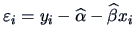
EXERCISE 3.11   Make a boxplot for the residuals $\varepsilon_{i}=y_{i}-\widehat\alpha - \widehat\beta x_{i}$ for the ``classic blue'' pullovers data. If there are outliers, identify them and run the linear regression again without them. Do you obtain a stronger influence of price on sales?

EXERCISE 3.12   Under what circumstances would you obtain the same coefficients from the linear regression lines of $Y$ on $X$ and of $X$ on $Y$?

EXERCISE 3.13   Treat the design of Example 3.14 as if there were thirty shops and not ten. Define $x_{i}$ as the index of the shop, i.e., $x_{i} = i, i = 1,2,\ldots, 30$. The null hypothesis is a constant regression line, $EY = \mu$. What does the alternative regression curve look like?

EXERCISE 3.14   Perform the test in Exercise 3.13 for the shop example with a $0.99$ significance level. Do you still reject the hypothesis of equal marketing strategies?

EXERCISE 3.15   Compute an approximate confidence interval for $\rho_{X_{2}X_{8}}$ in Example (3.2). Hint: start from a confidence interval for $\tanh^{-1}(\rho_{X_{2}X_{8}})$ and then apply the inverse transformation.

EXERCISE 3.16   In Example 3.2, using the exchange rate of 1 EUR = 106 JPY, compute the same empirical covariance using prices in Japanese Yen rather than in Euros. Is there a significant difference? Why?

EXERCISE 3.17   Why does the correlation have the same sign as the covariance?

EXERCISE 3.18   Show that $\mathop{\rm {rank}}(\data{H})=\mathop{\hbox{tr}}(\data{H})=n-1$.

EXERCISE 3.19   Show that $\data{X}_{*}=\data{H}\data{X}\data{D}^{-1/2}$ is the standardized data matrix, i.e.,
$\overline{x}_{*}=0$ and $\data{S}_{\data{X}_{*}}=\data{R}_{\data{X}}$.

EXERCISE 3.20   Compute for the pullovers data the regression of $X_{1}$ on $X_{2}, X_{3}$ and of $X_{1}$ on $X_{2}, X_{4}$. Which one has the better coefficient of determination?

EXERCISE 3.21   Compare for the pullovers data the coefficient of determination for the regression of $X_{1}$ on $X_{2}$ (Example 3.11), of $X_{1}$ on $X_{2}, X_{3}$ (Exercise 3.20) and of $X_{1}$ on $X_{2}, X_{3}, X_{4}$ (Example 3.15). Observe that this coefficient is increasing with the number of predictor variables. Is this always the case?

EXERCISE 3.22   Consider the ANOVA problem (Section 3.5) again. Establish the constraint Matrix $\data{A}$ for testing $\mu_{1}=\mu_{2}$. Test this hypothesis via an analog of (3.55) and (3.56).

EXERCISE 3.23   Prove (3.52). (Hint, let $f(\beta)=(y-x\beta)^{\top}(y-x\beta)$ and solve $\frac{\partial f(\beta)}{\partial \beta}=0$).

EXERCISE 3.24   Consider the linear model $Y=\data{X}{\beta}+\varepsilon$ where $\hat{\beta} =\arg \min\limits_{\beta}\varepsilon^{\top}\varepsilon$ is subject to the linear constraints $\data{A}\widehat\beta =a$ where $\data{A} (q\times p), (q \le p)$ is of rank $q$ and $a$ is of dimension $(q\times 1)$. Show that $\widehat\beta = \widehat\beta_{\textrm{{\small OLS}}}-(\data{X}^{\top}\data{X})... ...at\beta_{\textrm{{\small OLS}}}= (\data{X}^{\top}\data{X})^{-1}\data{X}^{\top}y$. (Hint, let $f(\beta,\lambda)=(y-x\beta)^{\top}(y-x\beta)-\lambda^{\top}(\data{A}\beta-a)$ where $\lambda \in \mathbb{R}^q$ and solve $\frac{\partial f(\beta ,\lambda)}{\partial \beta} =0$ and $\frac{\partial f(\beta ,\lambda)}{\partial \lambda}=0$).

EXERCISE 3.25   Compute the covariance matrix $\data{S}=\mathop{\mathit{Cov}}(\data{X})$ where $\data{X}$ denotes the matrix of observations on the counterfeit bank notes. Make a Jordan decomposition of $\data{S}$. Why are all of the eigenvalues positive?

EXERCISE 3.26   Compute the covariance of the counterfeit notes after they are linearly transformed by the vector $a=(1,1,1,1,1,1)^{\top}$.