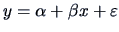
3.4 Linear Model for Two Variables
We have looked many times now at downward- and upward-sloping
scatterplots. What does the eye define here as slope? Suppose that we
can construct a line corresponding to the general direction of the
cloud. The sign of the slope of this line would correspond to the
upward and downward directions. Call the variable on the vertical
axis  and the one on the horizontal axis
  . A slope line is a linear
relationship between and :
. A slope line is a linear
relationship between and :
 |
(3.27) |
Here,  is the intercept and
  is the slope of the line. The
errors (or deviations from the line) are denoted as
is the slope of the line. The
errors (or deviations from the line) are denoted as
 and
are assumed to have zero mean and finite variance
and
are assumed to have zero mean and finite variance  .
The task of finding
.
The task of finding
 in (3.27) is
referred to as a linear adjustment.
in (3.27) is
referred to as a linear adjustment.
In Section 3.6 we shall derive estimators for
and more formally,
as well as accurately describe what a ``good'' estimator is. For now,
one may try to find a ``good'' estimator
 via graphical
techniques. A very common numerical and statistical
technique is to use those
via graphical
techniques. A very common numerical and statistical
technique is to use those
 and
and  that minimize:
 |
(3.28) |
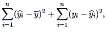
The solutions to this task are the estimators:
The variance of is:
 |
|
|
(3.31) |
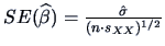
The standard error (SE) of the estimator is the square root of (3.31),
 |
|
|
(3.32) |
We can use this formula to test the hypothesis that
=0. In an application
the variance has to be estimated by an estimator
 that will be given below. Under a normality assumption
of the errors, the
that will be given below. Under a normality assumption
of the errors, the  -test for the hypothesis
  works as follows.
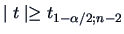
One computes the statistic
 |
|
|
(3.33) |
and rejects the hypothesis
at a 5% significance level if
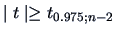 ,
where the 97.5% quantile of the Student's
,
where the 97.5% quantile of the Student's  distribution is clearly the 95% critical value
for the two-sided test.
For
distribution is clearly the 95% critical value
for the two-sided test.
For  , this can be replaced by 1.96, the 97.5% quantile of the
normal distribution.
An estimator
of will be given in the following.
, this can be replaced by 1.96, the 97.5% quantile of the
normal distribution.
An estimator
of will be given in the following.
EXAMPLE 3.10
Let us apply the linear regression model (
3.27) to the ``classic blue''
pullovers. The sales manager
believes that there is a strong dependence on the number of sales as a function
of price. He computes the regression line as shown in Figure
3.5.
Figure 3.5:
Regression of sales ( ) on price (
 ) of
pullovers.
) of
pullovers.
 MVAregpull.xpl
|
|
How good is this fit? This can be judged via goodness-of-fit
measures. Define
 |
(3.34) |
as the predicted value of  as a function of
  . With
  the
textile shop manager in the above example can predict sales as a
function of prices . The variation in the response variable is:
the
textile shop manager in the above example can predict sales as a
function of prices . The variation in the response variable is:
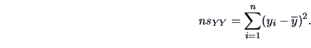 |
(3.35) |
The variation explained by the linear regression (3.27) with
the predicted values (3.34) is:
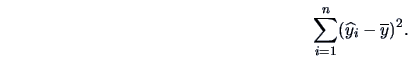 |
(3.36) |
The residual sum of squares, the minimum in (3.28), is
given by:
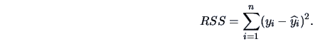 |
(3.37) |
An unbiased estimator
of is given by 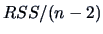 .
.
The following relation holds between (3.35)-(3.37):
The coefficient of determination is  :
:
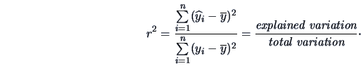 |
(3.39) |
The coefficient of determination increases with the proportion of
explained variation by the linear relation (3.27). In the extreme cases
where  , all of the variation is explained by the linear regression
(3.27). The other extreme,
, all of the variation is explained by the linear regression
(3.27). The other extreme,  , is where the empirical covariance is
 . The coefficient of determination can be rewritten as
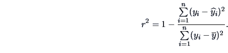 |
(3.40) |
From (3.39), it can be seen that in the linear regression
(3.27),
 is the square of the correlation between and .
EXAMPLE 3.11
For the above pullover example, we estimate
The coefficient of determination is
The textile shop manager concludes that sales are
not influenced very much by the price (in a linear way).
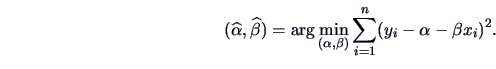
Figure 3.6:
Regression of sales ( ) on price (
 ) of
pullovers. The overall mean is given by the dashed line.
MVAregzoom.xpl
) of
pullovers. The overall mean is given by the dashed line.
MVAregzoom.xpl
|
|
The geometrical representation of formula (3.38) can be graphically
evaluated using Figure 3.6. This plot shows a section
of the linear
regression of the ``sales'' on ``price'' for the pullovers data.
The distance between any point and the overall mean is given by the distance
between the point and the regression line and the
distance between the regression line and the mean.
The sums of these two distances represent
the total variance
(solid blue lines from the observations to the overall mean), i.e.,
the explained variance (distance from the regression curve to the mean)
and the unexplained variance (distance from the observation to
the regression line), respectively.
In general the regression of on is different from that of
on . We will demonstrate this using once again the Swiss bank notes
data.
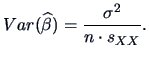
Figure 3.7:
Regression of  (upper inner frame)
on
(upper inner frame)
on  (lower inner frame) for genuine bank notes.
MVAregbank.xpl
(lower inner frame) for genuine bank notes.
MVAregbank.xpl
|
|
EXAMPLE 3.12
The least squares fit of the variables

(
) and

(
) from the genuine bank notes are calculated.
Figure
3.7 shows the fitted line if
is approximated
by a linear function of
.
In this case the parameters are
If we predict by a function of instead,
we would arrive at a different intercept and slope
The linear regression of on is given by minimizing (3.28), i.e.,
the vertical errors  . The linear regression of on
does the same but here the errors to be minimized in the least squares
sense are measured horizontally. As seen in Example 3.12, the two
least squares lines are different although both measure (in a certain
sense) the slope of the cloud of points.
. The linear regression of on
does the same but here the errors to be minimized in the least squares
sense are measured horizontally. As seen in Example 3.12, the two
least squares lines are different although both measure (in a certain
sense) the slope of the cloud of points.
As shown in the next example, there is still one other way to measure the main
direction of a cloud of points: it is related to the spectral decomposition
of covariance matrices.
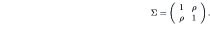
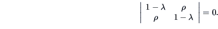
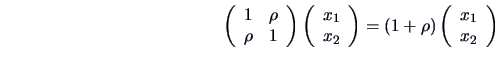
EXAMPLE 3.13
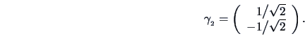
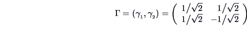
Suppose that we have the following covariance matrix:
Figure
3.8 shows a scatterplot of a sample of two normal random
variables with such a covariance matrix (with

).
Figure 3.8:
Scatterplot for a sample of two
correlated normal random variables (sample size  , ).
MVAcorrnorm.xpl
, ).
MVAcorrnorm.xpl
|
|
The eigenvalues of  are, as was shown in Example 2.4,
solutions to:
are, as was shown in Example 2.4,
solutions to:
Hence,

and

. Therefore
.
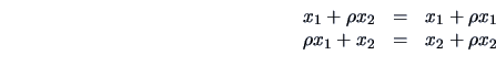
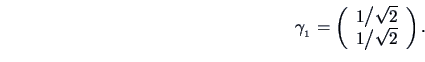
The eigenvector corresponding to
can be computed from
the system of linear equations:
or
and thus
The first (standardized) eigenvector is
The direction of this eigenvector is the diagonal in Figure
3.8 and captures the main variation in this direction. We
shall come back to this interpretation in Chapter
9.
The second eigenvector (orthogonal to

) is
So finally
and we can check our calculation by
The first eigenvector captures the main direction of a point cloud.
The linear regression of on and on accomplished, in a
sense, the same thing. In general
the direction of the eigenvector and the least squares slope are
different. The reason is that the least squares
estimator minimizes either vertical or horizontal errors (in 3.28),
whereas the first eigenvector corresponds to a minimization
that is orthogonal to the eigenvector (see Chapter 9).
Summary

-
The linear regression
 models a linear
relation between two one-dimensional variables.
models a linear
relation between two one-dimensional variables.
-
The sign of the slope is the same as that of the
covariance and the correlation of and .
-
A linear regression predicts values of given a
possible observation of .
-
The coefficient of determination measures the amount of
variation in which is explained by a linear regression on .
-
If the coefficient of determination is = 1,
then all points lie on one line.
-
The regression line of on and the regression line of on
are in general different.
-
The -test for the hypothesis = 0 is
 , where
 .
.
-
The -test rejects the null hypothesis = 0
at the level of significance
if
 where
where
 is the
  quantile of the Student's
-distribution with
quantile of the Student's
-distribution with  degrees of freedom.
-
The standard error
 increases/decreases with less/more
spread in the variables.
increases/decreases with less/more
spread in the variables.
-
The direction of the first eigenvector of the covariance matrix
of a two-dimensional point cloud is different from the least squares
regression line.
![\includegraphics[width=1\defpicwidth]{MVAregzoom.ps}](mvahtmlimg860.gif)
![\includegraphics[width=1\defpicwidth]{MVAregbank.ps}](mvahtmlimg861.gif)
![\includegraphics[width=1\defpicwidth]{corrnorm.ps}](mvahtmlimg867.gif)
![\includegraphics[width=1\defpicwidth]{MVAregpull.ps}](mvahtmlimg840.gif)