11.2 The Proximity between Objects

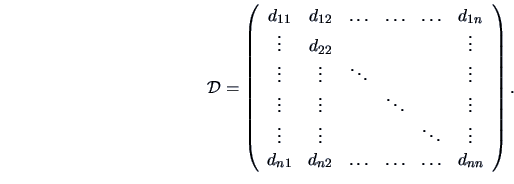
The starting point of a cluster analysis is a data matrix $\data{X}(n\times p)$ with $n$ measurements (objects) of $p$ variables. The proximity (similarity) among objects is described by a matrix $\data{D}(n\times n)$

$${{\data{D}}} = \left(\begin{array}{cccccc} d_{11}&d_{12}&\ld... ...{n1}&d_{n2}&\ldots &\ldots &\ldots &d_{nn}\end{array}\right).$$ (11.1)

The matrix $\data{D}$ contains measures of similarity or dissimilarity among the $n$ objects. If the values $d_{ij}$ are distances, then they measure dissimilarity. The greater the distance, the less similar are the objects. If the values $d_{ij}$ are proximity measures, then the opposite is true, i.e., the greater the proximity value, the more similar are the objects. A distance matrix, for example, could be defined by the $L_{2}$-norm: $d_{ij} = \Vert x_{i} - x_{j} \Vert _{2}$, where $x_{i}$ and $x_{j}$ denote the rows of the data matrix $\data{X}$. Distance and similarity are of course dual. If $d_{ij}$ is a distance, then $d'_{ij}=\max_{i,j}\{d_{ij}\}-d_{ij}$ is a proximity measure.

The nature of the observations plays an important role in the choice of proximity measure. Nominal values (like binary variables) lead in general to proximity values, whereas metric values lead (in general) to distance matrices. We first present possibilities for $\data{D}$ in the binary case and then consider the continuous case.

Similarity of objects with binary structure

In order to measure the similarity between objects we always compare pairs of observations $(x_{i}, x_{j})$ where $x_{i}^{\top}=(x_{i1},\ldots,x_{ip})$, $x_{j}^{\top}=(x_{j1},\ldots,x_{jp})$, and $x_{ik}, x_{jk} \in \{0,1\}$. Obviously there are four cases:

$$\begin{eqnarray*} &&x_{ik}=x_{jk}=1,\\ &&x_{ik}=0, x_{jk}=1,\\ &&x_{ik}=1, x_{jk}=0,\\ &&x_{ik}=x_{jk}=0. \end{eqnarray*}$$

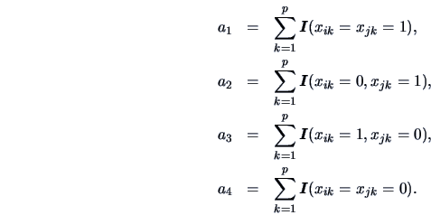
Define

$$\begin{eqnarray*} a_{1}&=&\sum_{k=1}^p {\boldsymbol{I}}{(x_{ik}=x_{jk}=1)},\\ a... ...},\\ a_{4}&=&\sum_{k=1}^p {\boldsymbol{I}}{(x_{ik}=x_{jk}=0)}. \end{eqnarray*}$$

Note that each $a_{\ell},\ \ell=1,\ldots,4$, depends on the pair $(x_{i}, x_{j})$.

The following proximity measures are used in practice:

$$d_{ij}=\frac{a_{1}+\delta a_{4}}{a_{1}+\delta a_{4}+\lambda(a_{2}+a_{3})}$$ (11.2)

where $\delta$ and $\lambda$ are weighting factors. Table 11.1 shows some similarity measures for given weighting factors.

Table 11.1: The common similarity coefficients.

Name	$\delta$	$\lambda$	Definition
Jaccard	0	1	$\frac{\displaystyle a_{1}}{\displaystyle a_{1}+a_{2}+a_{3}}$
Tanimoto	1	2	$\frac{\displaystyle a_{1}+a_{4}}{\displaystyle a_{1}+2(a_{2}+a_{3})+a_{4}}$
Simple Matching (M)	1	1	$\frac{\displaystyle a_{1}+a_{4}}{\displaystyle p}$
Russel and Rao (RR)	-	-	$\frac{\displaystyle a_{1}}{\displaystyle p}$
Dice	0	0.5	$\frac{\displaystyle 2a_{1}}{\displaystyle 2a_{1}+(a_{2}+a_{3})}$
Kulczynski	-	-	$\frac{\displaystyle a_{1}}{\displaystyle a_{2}+a_{3}}$

These measures provide alternative ways of weighting mismatchings and positive (presence of a common character) or negative (absence of a common character) matchings. In principle, we could also consider the Euclidian distance. However, the disadvantage of this distance is that it treats the observations $0$ and $1$ in the same way. If $x_{ik}=1$ denotes, say, knowledge of a certain language, then the contrary, $x_{ik}=0$ (not knowing the language) should eventually be treated differently.

EXAMPLE 11.1   Let us consider binary variables computed from the car data set (Table B.7). We define the new binary data by

$$y_{ik}= \left\{ \begin{array}{ll} 1&\quad\textrm{if }x_{ik}>... ...ine{x}_{k},\\ 0&\quad\textrm{otherwise,} \end{array} \right.$$

for $i=1,\ldots ,n$ and $k = 1,\ldots, p$. This means that we transform the observations of the $k$-th variable to $1$ if it is larger than the mean value of all observations of the $k$-th variable. Let us only consider the data points 17 to 19 (Renault 19, Rover and Toyota Corolla) which lead to $(3\times 3)$ distance matrices. The Jaccard measure gives the similarity matrix

$$\data{D}= \left(\begin{array}{ccc} 1.000 & 0.000 & 0.333\\ & 1.000 & 0.250\\ & & 1.000 \end{array}\right),$$

the Tanimoto measure yields

$$\data{D}= \left(\begin{array}{ccc} 1.000 & 0.231 & 0.600\\ & 1.000 & 0.455\\ & & 1.000 \end{array}\right),$$

whereas the Single Matching measure gives

$$\data{D}= \left(\begin{array}{ccc} 1.000 & 0.375 & 0.750 \\ & 1.000 & 0.625 \\ & & 1.000 \end{array}\right).$$

Distance measures for continuous variables

A wide variety of distance measures can be generated by the $L_{r}$-norms, $r \ge 1$,

$$d_{ij} = \vert\vert x_{i}-x_{j}\vert\vert _{r} = \left \{ \sum^p_{k=1} \vert x_{ik}-x_{jk}\vert^r \right \}^{1/r}.$$ (11.3)

Here $x_{ik}$ denotes the value of the $k$-th variable on object $i$. It is clear that $d_{ii} = 0$ for $i=1,\ldots ,n$. The class of distances (11.3) for varying $r$ measures the dissimilarity of different weights. The $L_{1}$-metric, for example, gives less weight to outliers than the $L_{2}$-norm (Euclidean norm). It is common to consider the squared $L_{2}$-norm.

EXAMPLE 11.2   Suppose we have $x_{1} =(0,0),\, x_{2} = (1,0)$ and $x_{3} =(5,5)$. Then the distance matrix for the $L_{1}$-norm is

$$\data{D}_{1} = \left( \begin{array}{rrr} 0 & 1 & 10 \\ 1 & 0 & 9 \\ 10 & 9 & 0 \end{array} \right),$$

and for the squared $L_{2}$- or Euclidean norm

$$\data{D}_{2} = \left ( \begin{array}{rrr} 0 & 1 & 50 \\ 1 & 0 & 41\\ 50 & 41 & 0 \end{array} \right ).$$

One can see that the third observation $x_{3}$ receives much more weight in the squared $L_{2}$-norm than in the $L_{1}$-norm.

An underlying assumption in applying distances based on $L_{r}$-norms is that the variables are measured on the same scale. If this is not the case, a standardization should first be applied. This corresponds to using a more general $L_{2}$- or Euclidean norm with a metric $\data{A}$, where $\data{A}>0$ (see Section 2.6):

$$d^2_{ij}=\Vert x_{i}-x_{j}\Vert _{\data{A}} = (x_{i}-x_{j})^{\top}\data{A}(x_{i}-x_{j}).$$ (11.4)

$L_{2}$-norms are given by $\data{A}=\data{I}_{p}$, but if a standardization is desired, then the weight matrix $\data{A}= \mathop{\hbox{diag}}(s_{X_{1}X_{1}}^{-1},\ldots,s_{X_{p}X_{p}}^{-1})$ may be suitable. Recall that $s_{X_{k}X_{k}}$ is the variance of the $k$-th component. Hence we have

$$d^2_{ij}=\sum_{k=1}^p \frac{ (x_{ik}-x_{jk})^2 }{s_{X_{k}X_{k}}}.$$ (11.5)

Here each component has the same weight in the computation of the distances and the distances do not depend on a particular choice of the units of measure.

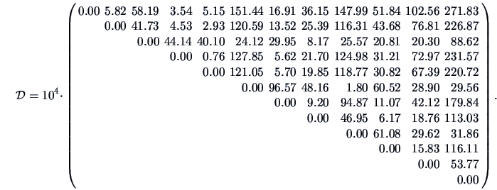
EXAMPLE 11.3   Consider the French Food expenditures (Table B.6). The Euclidean distance matrix (squared $L_{2}$-norm) is

$${\arraycolsep2pt \data{D}=10^4\cdotp\left(\begin{array}{rrr... ...& 53.77\\ & & & & & & & & & & & 0.00 \end{array}\right). }$$

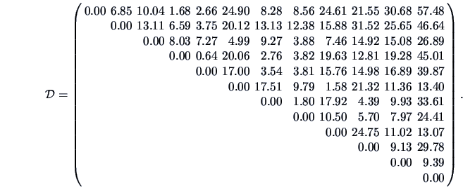
Taking the weight matrix $\data{A}=\mathop{\hbox{diag}}(s_{X_{1}X_{1}}^{-1},\ldots,s_{X_{7}X_{7}}^{-1})$, we obtain the distance matrix (squared $L_{2}$-norm)

$${\arraycolsep2pt \data{D}=\left(\begin{array}{rrrrrrrrrrrr}... ...0& 9.39\\ & & & & & & & & & & & 0.00 \end{array}\right). }$$ (11.6)

When applied to contingency tables, a $\chi^2$-metric is suitable to compare (and cluster) rows and columns of a contingency table.

If $\data{X}$ is a contingency table, row $i$ is characterized by the conditional frequency distribution $\frac{x_{ij}}{x_{i\bullet}}$, where $x_{i \bullet} = \sum_{j=1}^p x_{ij}$ indicates the marginal distributions over the rows: $\frac{x_{i \bullet}}{x_{\bullet \bullet}}, \; x_{\bullet \bullet} = \sum_{i=1}^n x_{i \bullet}$. Similarly, column $j$ of $\data{X}$ is characterized by the conditional frequencies $\frac{x_{ij}}{x_{\bullet j}}$, where $x_{\bullet j} = \sum_{i=1}^n x_{ij}$. The marginal frequencies of the columns are $\frac{x_{\bullet j}}{x_{\bullet \bullet}}$.

The distance between two rows, $i_1$ and $i_2$, corresponds to the distance between their respective frequency distributions. It is common to define this distance using the $\chi^2$-metric:

$$d^2(i_1, i_2) = \sum_{j=1}^p \frac{1}{\left( \frac{x_{\bull... ...i_1 \bullet}} - \frac{x_{i_2 j}}{x_{i_2 \bullet}} \right)^2.$$ (11.7)

Note that this can be expressed as a distance between the vectors $x_{1} = \left( \frac{x_{i_1 j}}{x_{\bullet \bullet}} \right)$ and $x_{2}= \left( \frac{x_{i_2 j}}{x_{\bullet \bullet}} \right)$ as in (11.4) with weighting matrix $\data{A} =\left\{ diag \left( \frac{x_{\bullet j}}{x_{\bullet \bullet}} \right)\right\}^{-1}$. Similarly, if we are interested in clusters among the columns, we can define:

$$d^2(j_1, j_2) = \sum_{i=1}^n \frac{1}{\left( \frac{x_{i \bul... ..._{\bullet j_1}} - \frac{x_{i j_2}}{x_{\bullet j_2}} \right)^2.$$

Apart from the Euclidean and the $L_{r}$-norm measures one can use a proximity measure such as the Q-correlation coefficient

$$d_{ij} = \frac {\sum^p_{k=1}(x_{ik}-\overline{x}_{i})(x_{jk... ...^2 \sum^p_{k=1}(x_{jk}-\overline{x}_{j})^2 \right \}^{1/2}}.$$ (11.8)

Here $\overline{x}_{i}$ denotes the mean over the variables $(x_{i1}, \ldots, x_{ip})$.

Summary

$\ast$

The proximity between data points is measured by a distance or similarity matrix $\data{D}$ whose components $d_{ij}$ give the similarity coefficient or the distance between two points $x_{i}$ and $x_{j}$.

$\ast$

A variety of similarity (distance) measures exist for binary data (e.g., Jaccard, Tanimoto, Simple Matching coefficients) and for continuous data (e.g., $L_{r}$-norms).

$\ast$

The nature of the data could impose the choice of a particular metric $\data{A}$ in defining the distances (standardization, $\chi^2$-metric etc.).