2.6 Geometrical Aspects

Distance

Let $x,y\in \mathbb{R}^p$. A distance $d$ is defined as a function

$$d: \mathbb{R}^{2p}\to \mathbb{R}_+ \quad \textrm{which fulfil... ...(x,y)\le d(x,z)+d(z,y) & \forall x,y,z\\ \end{array}\right. .$$

A Euclidean distance $d$ between two points $x$ and $y$ is defined as

$$d^2(x,y)=(x-y)^{T} \data{A}(x-y)$$ (2.32)

where $\data{A}$ is a positive definite matrix $(\data{A}>0)$. $\data{A}$ is called a metric.

EXAMPLE 2.10   A particular case is when $\data{A}=\data{I}_p$, i.e.,

$$d^2 (x,y)=\sum_{i=1}^p {(x_i-y_i)}^2.$$ (2.33)

Figure 2.1 illustrates this definition for $p=2$.

Note that the sets $E_d=\{x \in \mathbb{R}^p \mid (x-x_0)^{\top}(x-x_0)=d^2 \}$ , i.e., the spheres with radius $d$ and center $x_0$, are the Euclidean ${\data{I}}_p$ iso-distance curves from the point $x_0$ (see Figure 2.2).

Figure 2.1: Distance $d$.

Figure 2.2: Iso-distance sphere.

The more general distance (2.32) with a positive definite matrix $\data{A} \ (\data{A}>0)$ leads to the iso-distance curves

$$E_d =\{ x \in \mathbb{R}^p \mid (x-x_0)^{\top}\data{A}(x-x_0)=d^2 \},$$ (2.34)

i.e., ellipsoids with center $x_0$, matrix $\data{A}$ and constant $d$ (see Figure 2.3).

Figure 2.3: Iso-distance ellipsoid.

Let $\gamma_1 , \gamma_2 ,..., \gamma_p$ be the orthonormal eigenvectors of $\data{A}$ corresponding to the eigenvalues $\lambda_1 \ge \lambda_2 \ge ... \ge \lambda_p$. The resulting observations are given in the next theorem.

THEOREM 2.7  

(i)

The principal axes of $E_d$ are in the direction of $\gamma_i ; \ i=1,\ldots,p$.

(ii)

The half-lengths of the axes are $\sqrt{ \frac{d^2} {\lambda_i} }$; $i = 1,\ldots ,p$.

(iii)

The rectangle surrounding the ellipsoid $E_d$ is defined by the following inequalities:

$$x_{0i} - \sqrt{d^2 a^{ii}} \le x_i \le x_{0i} + \sqrt{d^2 a^{ii}}, \quad i=1,\ldots,p,$$

where $a^{ii}$ is the $(i,i)$ element of $\data{A}^{-1}$. By the rectangle surrounding the ellipsoid $E_d$ we mean the rectangle whose sides are parallel to the coordinate axis.

It is easy to find the coordinates of the tangency points between the ellipsoid and its surrounding rectangle parallel to the coordinate axes. Let us find the coordinates of the tangency point that are in the direction of the $j$-th coordinate axis (positive direction).

For ease of notation, we suppose the ellipsoid is centered around the origin $(x_0=0)$. If not, the rectangle will be shifted by the value of $x_0$.

The coordinate of the tangency point is given by the solution to the following problem:

$$x=\arg \max_{x^{\top}\data{A} x = d^2} e^{\top}_j x$$ (2.35)

where $e^{\top}_j$ is the $j$-th column of the identity matrix $\data{I}_p$. The coordinate of the tangency point in the negative direction would correspond to the solution of the min problem: by symmetry, it is the opposite value of the former.

The solution is computed via the Lagrangian $L= e^{\top}_j x-\lambda(x^{\top}\data{A} x - d^2)$ which by (2.23) leads to the following system of equations:

$$\frac{\partial L}{\partial x}= e_j - 2\lambda \data{A} x =0$$ (2.36)

$$\frac{\partial L}{\partial \lambda}=x^{T} \data{A} x - d^2=0.$$ (2.37)

This gives $x=\frac{1}{2\lambda} \data{A}^{-1} e_j$, or componentwise

$$x_i=\frac{1}{2\lambda} a^{ij},\; i=1,\ldots,p$$ (2.38)

where $a^{ij}$ denotes the $(i,j)$-th element of $\data{A}^{-1}$.

Premultiplying (2.36) by $x^{\top}$, we have from (2.37):

$$x_j=2\lambda d^2.$$

Comparing this to the value obtained by (2.38), for $i=j$ we obtain $2\lambda=\sqrt{\frac{a^{jj}}{d^2}}$. We choose the positive value of the square root because we are maximizing $e_j^{\top} x$. A minimum would correspond to the negative value. Finally, we have the coordinates of the tangency point between the ellipsoid and its surrounding rectangle in the positive direction of the $j$-th axis:

$$x_i = \sqrt{\frac{d^2}{a^{jj}}}\; a^{ij},\; i=1,\ldots, p.$$ (2.39)

The particular case where $i=j$ provides statement $(iii)$ in Theorem 2.7.

Remark: usefulness of Theorem 2.7

Theorem 2.7 will prove to be particularly useful in many subsequent chapters. First, it provides a helpful tool for graphing an ellipse in two dimensions. Indeed, knowing the slope of the principal axes of the ellipse, their half-lengths and drawing the rectangle inscribing the ellipse allows one to quickly draw a rough picture of the shape of the ellipse.

In Chapter 7, it is shown that the confidence region for the vector $\mu$ of a multivariate normal population is given by a particular ellipsoid whose parameters depend on sample characteristics. The rectangle inscribing the ellipsoid (which is much easier to obtain) will provide the simultaneous confidence intervals for all of the components in $\mu$.

In addition it will be shown that the contour surfaces of the multivariate normal density are provided by ellipsoids whose parameters depend on the mean vector and on the covariance matrix. We will see that the tangency points between the contour ellipsoids and the surrounding rectangle are determined by regressing one component on the $(p-1)$ other components. For instance, in the direction of the $j$-th axis, the tangency points are given by the intersections of the ellipsoid contours with the regression line of the vector of $(p-1)$ variables (all components except the $j$-th) on the $j$-th component.

Norm of a Vector

Consider a vector $x\in \mathbb{R}^p$. The norm or length of $x$ (with respect to the metric $\data{I}_p$) is defined as

$$\Vert x \Vert = d(0,x)=\sqrt{x^{\top}x}.$$

If $\Vert x \Vert =1,x$ is called a unit vector. A more general norm can be defined with respect to the metric $\data{A}$:

$$\Vert x \Vert _{\data{A}} = \sqrt{x^{\top}\data{A}x}.$$

Angle between two Vectors

Consider two vectors $x$ and $y \in \mathbb{R}^p$. The angle $\theta$ between $x$ and $y$ is defined by the cosine of $\theta$:

$$\cos \theta = \frac{x^{\top}y}{\Vert x \Vert \ \Vert y \Vert},$$ (2.40)

see Figure 2.4. Indeed for $p=2$, $x={\displaystyle {x_1 \choose x_2}}$ and $y={\displaystyle {y_1 \choose y_2}}$, we have

$$\begin{array}{rclrcl} \Vert x \Vert \cos \theta_{1} &=&x_1\ ... ...} &=&x_2\ ;& \Vert y \Vert \sin \theta_{2} &=&y_2, \end{array}$$ (2.41)

therefore,

$$\cos\theta=\cos\theta_{1}\cos\theta_{2}+\sin\theta_{1}\sin\th... ...rt y \Vert} =\frac{x^{\top}y}{\Vert x \Vert \ \Vert y \Vert}\ .$$

Figure 2.4: Angle between vectors.

REMARK 2.1   If $x^{\top}y=0$, then the angle $\theta$ is equal to ${\displaystyle \frac{\pi}{2}}$. From trigonometry, we know that the cosine of $\theta$ equals the length of the base of a triangle ($\vert\vert p_x\vert\vert$) divided by the length of the hypotenuse ($\vert\vert x\vert\vert$). Hence, we have

$$\vert\vert p_x\vert\vert = \vert\vert x\vert\vert \vert \cos \theta \vert=\frac{\vert x^{\top}y\vert}{\Vert y \Vert} ,$$ (2.42)

where $p_x$ is the projection of $x$ on $y$ (which is defined below). It is the coordinate of $x$ on the $y$ vector, see Figure 2.5.

Figure 2.5: Projection.

The angle can also be defined with respect to a general metric $\data{A}$

$$\cos \theta=\frac{x^{\top}\data{A}y} {\Vert x \Vert _{\data{A}}\ \Vert y \Vert _{\data{A}}}.$$ (2.43)

If $\cos \theta =0$ then $x$ is orthogonal to $y$ with respect to the metric $\data{A}$.

EXAMPLE 2.11   Assume that there are two centered (i.e., zero mean) data vectors. The cosine of the angle between them is equal to their correlation (defined in (3.8))! Indeed for $x$ and $y$ with $\overline{x} = \overline{y} = 0$ we have

$$r_{XY} = \frac{\sum x_{i}y_{i}}{\sqrt{\sum x_{i}^2 \sum y_{i}^2}} = \cos\theta$$

according to formula (2.40).

Rotations

When we consider a point $x\in \mathbb{R}^p$, we generally use a $p$-coordinate system to obtain its geometric representation, like in Figure 2.1 for instance. There will be situations in multivariate techniques where we will want to rotate this system of coordinates by the angle $\theta$.

Consider for example the point $P$ with coordinates $x=(x_1, x_2)^{\top}$ in $\mathbb{R}^2$ with respect to a given set of orthogonal axes. Let $\Gamma$ be a $(2\times 2)$ orthogonal matrix where

$$\Gamma=\left(\begin{array}{cc} \cos \theta &\sin \theta \\ -\sin \theta &\cos \theta \end{array} \right).$$ (2.44)

If the axes are rotated about the origin through an angle $\theta$ in a clockwise direction, the new coordinates of $P$ will be given by the vector $y$

$$y=\Gamma \,x,$$ (2.45)

and a rotation through the same angle in a counterclockwise direction gives the new coordinates as

$$y=\Gamma^{\top} \,x.$$ (2.46)

More generally, premultiplying a vector $x$ by an orthogonal matrix $\Gamma$ geometrically corresponds to a rotation of the system of axes, so that the first new axis is determined by the first row of $\Gamma$. This geometric point of view will be exploited in Chapters 9 and 10.

Column Space and Null Space of a Matrix

Define for $\data{X}(n\times p)$

$$Im(\data{X}) \stackrel{def}{=} {C}(\data{X}) =\{x\in \mathbb{... ...\exists a \in \mathbb{R}^p \textrm{ so that } \data{X}a=x \},$$

the space generated by the columns of $\data{X}$ or the column space of $\data{X}$. Note that ${C}(\data{X}) \subseteq \mathbb{R}^n$ and $\textrm{dim}\{{C}(\data{X})\}=\mathop{\rm {rank}}(\data{X})=r\le \min(n,p).$

$$Ker(\data{X})\stackrel{def}{=} {N}(\data{X})=\{y\in \mathbb{R}^p \mid \data{X}y=0 \}$$

is the null space of $\data{X}$. Note that ${N}(\data{X}) \subseteq \mathbb{R}^p$ and that $\textrm{dim}\{{N}(\data{X})\}=p-r.$

REMARK 2.2   ${N}(\data{X}^{\top})$ is the orthogonal complement of ${C}(\data{X})$ in $\mathbb{R}^n$, i.e., given a vector $b \in \mathbb{R}^n$ it will hold that $x^{\top}b=0$ for all $x \in {C}(\data{X})$, if and only if $b \in {N}(\data{X}^{\top})$.

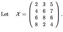
EXAMPLE 2.12   ${\textrm{Let }}\quad {\data X}=\left(\begin{array}{ccc}2&3&5\\ 4&6&7\\ 6&8&6\\ 8&2&4\end{array}\right).$ It is easy to show (e.g. by calculating the determinant of $\data{X}$) that $\mathop{\rm {rank}}({\data X})=3$. Hence, the columns space of $\data{X}$ is ${C}(\data{X})=\mathbb{R}^3$. The null space of $\data{X}$ contains only the zero vector $(0,0,0)^{\top}$ and its dimension is equal to $\mathop{\rm {rank}}({\data X})-3=0$.

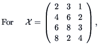
${\textrm{For }}\quad {\data X}=\left(\begin{array}{ccc}2&3&1\\ 4&6&2\\ 6&8&3\\ 8&2&4\end{array}\right),$ the third column is a multiple of the first one and the matrix ${\data X}$ cannot be of full rank. Noticing that the first two columns of ${\data X}$ are independent, we see that $\mathop{\rm {rank}}({\data X})=2$. In this case, the dimension of the columns space is 2 and the dimension of the null space is 1.

Projection Matrix

A matrix $\data{P}(n \times n)$ is called an (orthogonal) projection matrix in $\mathbb{R}^n$ if and only if $\data{P}=\data{P}^{\top}=\data{P}^2$ ($\data{P}$ is idempotent). Let $b \in \mathbb{R}^n$. Then $a=\data{P}b$ is the projection of $b$ on ${C}(\data{P})$.

Projection on ${C}(\data{X})$

Consider $\data{X}(n\times p)$ and let

$$\data{P}=\data{X} (\data{X}^{\top}\data{X})^{-1}\data{X}^{\top}$$ (2.47)

and $\data{Q}=\data{I}_n-\data{P}$. It's easy to check that $\data{P}$ and $\data{Q}$ are idempotent and that

$$\data{P}\data{X}=\data{X}\textrm{ and }\data{Q}\data{X}=0.$$ (2.48)

Since the columns of $\data{X}$ are projected onto themselves, the projection matrix $\data{P}$ projects any vector $b \in \mathbb{R}^n$ onto ${C}(\data{X})$. Similarly, the projection matrix $\data{Q}$ projects any vector $b \in \mathbb{R}^n$ onto the orthogonal complement of ${C}(\data{X})$.

THEOREM 2.8   Let ${\data{P}}$ be the projection (2.47) and ${\data{Q}}$ its orthogonal complement. Then:

(i)

$x=\data{P}b \Rightarrow x \in {C}(\data{X})$,

(ii)

$y=\data{Q}b \Rightarrow y^{\top}x=0 \ \forall x \in {C}(\data{X})$.

PROOF:
(i) holds, since $x=\data{X}(\data{X}^{\top}\data{X})^{-1}\data{X}^{\top}b=\data{X}a$, where $a=(\data{X}^{\top}\data{X})^{-1}\data{X}^{\top}b \in \mathbb{R}^p$.
(ii) follows from $y=b-\data{P}b$ and $x=\data{X}a \Rightarrow y^{\top}x=b^{\top}\data{X}a-b^{\top}\data{X}(\data{X}^{\top}\data{X})^{-1} \data{X}^{\top}\data{X}a=0$. ${\Box}$

REMARK 2.3   Let $x,y \in \mathbb{R}^n$ and consider $p_x \in \mathbb{R}^n$, the projection of $x$ on $y$ (see Figure 2.5). With $\data{X}=y$ we have from (2.47)

$$p_x=y(y^{\top}y)^{-1}y^{\top}x=\frac{y^{\top}x}{\Vert y \Vert^2}\ y$$ (2.49)

and we can easily verify that

$$\Vert p_x\Vert=\sqrt{p_x^{\top}p_x}=\frac{\vert y^{\top}x\vert}{\Vert y\Vert}.$$

See again Remark 2.1.

Summary

$\ast$

A distance between two $p$-dimensional points $x$ and $y$ is a quadratic form $(x-y)^{\top}\data{A}(x-y)$ in the vectors of differences $(x-y)$. A distance defines the norm of a vector.

$\ast$

Iso-distance curves of a point $x_{0}$ are all those points that have the same distance from $x_{0}$. Iso-distance curves are ellipsoids whose principal axes are determined by the direction of the eigenvectors of ${\data A}$. The half-length of principal axes is proportional to the inverse of the roots of the eigenvalues of $\data{A}$.

$\ast$

The angle between two vectors $x$ and $y$ is given by $\cos \theta = \frac{x^{\top}\data{A}y}{\Vert x \Vert _{\data{A}} \ \Vert y \Vert _{\data{A}}}$ w.r.t. the metric $\data{A}$.

$\ast$

For the Euclidean distance with ${\data{A}}={\data{I}}$ the correlation between two centered data vectors $x$ and $y$ is given by the cosine of the angle between them, i.e., $\cos \theta = r_{XY}$.

$\ast$

The projection $\data{P}=\data{X} (\data{X}^{\top}\data{X})^{-1}\data{X}^{\top}$ is the projection onto the column space $C(\data{X})$ of $\data{X}$.

$\ast$

The projection of $x\in \mathbb{R}^n$ on $y \in \mathbb{R}^n$ is given by $p_x=\frac{y^{\top}x}{\Vert y\Vert^2}y.$