Throughout the entire section
 are unbounded,
i.i.d. random variables with distribution function
are unbounded,
i.i.d. random variables with distribution function  .
.
Notation:
 and
and
 represent the order
statistics, that is, the data is sorted
according to increasing or decreasing size. Obviously then
represent the order
statistics, that is, the data is sorted
according to increasing or decreasing size. Obviously then
 etc.
etc.
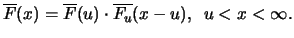
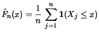
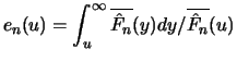
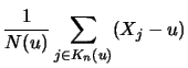
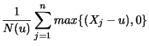
Definition 18.7 (Empirical Average Excess Function)
Let
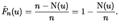
be the index of the
observations outside of the threshold

, and let
be their total number and
the
empirical distribution function,

.
is called the
empirical average excess function.
 estimates the average excess function
  from Section
17.1.
from Section
17.1.
As an explorative data analysis the following graphs will be
considered:
Plot of the probability distribution function |
|
 |
|
| Quantile plot |
|
 |
|
| Average excess plot |
|
 |
|
If the original model assumptions, that is the distribution of
the data, is correct, then the first two graphs should be
approximately linear. If this is not the case, then the
distribution assumptions must be changed. On the other hand, due
to Theorem 17.5, b) the average excess plot is for
size  approximately linear with a slope
 if
belongs to the maximum domain of attraction of a Fréchet
distribution
if
belongs to the maximum domain of attraction of a Fréchet
distribution
 for
for
 , i.e. with a finite
expectation.
, i.e. with a finite
expectation.
As an example consider the daily returns of the exchange rate
between the Yen and the U.S. dollar from December 1, 1978 to
January 31, 1991 in Figure 17.4. Figure 17.5 shows
the plot of the probability distribution function and the quantile
plot for the pdf
 of the standard normal. The
deviations from the straight line clearly shows that the data is
not normally distributed. Figure 17.6 shows again the average
excess plot of the data.
of the standard normal. The
deviations from the straight line clearly shows that the data is
not normally distributed. Figure 17.6 shows again the average
excess plot of the data.
Fig.:
Empirical mean excess function (solid line), GP mean excess function for Hill estimator (dotted line) and moment estimator (broken line).
 SFEjpyusd.xpl
|
|
In this section and the following we will take a look at
estimators for extreme value characteristics such as the
exceedance probabilities
 for values
 or the extreme quantile
 for
for

First, we only consider distributions that are contained in
the MDA of a GEV distribution
 . The
corresponding random variables are thus unbounded.
. The
corresponding random variables are thus unbounded.
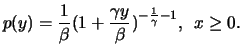
Definition 18.8 (Excess)
Let

and

be, as before, the index and total
number of observations beyond the threshold
respectively. The
excess beyond the threshold
is defined as the random
variables
with
The excesses
 describe by how much the
observations, which are larger than , go beyond the threshold
. The POT method (peaks-over-threshold
method) assumes that these excesses are the basic information
source for the initial data. From the definition it immediately
follows that
describe by how much the
observations, which are larger than , go beyond the threshold
. The POT method (peaks-over-threshold
method) assumes that these excesses are the basic information
source for the initial data. From the definition it immediately
follows that
 are i.i.d. random variables
with distribution
are i.i.d. random variables
with distribution  given their random total number
,
i.e., the excess distribution from Definition 17.5 is
the actual distribution of the excesses. Due to Theorem
17.6 it also holds that
given their random total number
,
i.e., the excess distribution from Definition 17.5 is
the actual distribution of the excesses. Due to Theorem
17.6 it also holds that
 for a GP distribution
 and all sufficiently large .
Let's first consider the problem of estimating the exceedance
probability
 for large . A natural estimator
is
for large . A natural estimator
is
 , the cdf at is replaced with the
empirical distribution function. For large , however, the
empirical distribution function varies a lot, because it is
determined by the few extreme observations which are located
around . The effective size of the sub-sample of extreme, large
observations is too small to use a pure non-parametric estimator
such as the empirical distribution function. Therefore, we use the
following relationship among the extreme exceedance probability
, the exceedance probability
, the cdf at is replaced with the
empirical distribution function. For large , however, the
empirical distribution function varies a lot, because it is
determined by the few extreme observations which are located
around . The effective size of the sub-sample of extreme, large
observations is too small to use a pure non-parametric estimator
such as the empirical distribution function. Therefore, we use the
following relationship among the extreme exceedance probability
, the exceedance probability
 for a large, but not extremely large threshold and the excess
distribution. Due to Definition 17.5 the excess
distribution is
for a large, but not extremely large threshold and the excess
distribution. Due to Definition 17.5 the excess
distribution is
| |
|
 i.e. i.e. |
|
| |
|
 |
(18.4) |
For large and using Theorem 17.6 we can approximate
with
 for appropriately chosen
 .
.  is replaced with the empirical distribution
function
is replaced with the empirical distribution
function
 at the threshold , for which due to the
definition of
it holds that
For itself this is a useful approximation, but not for the
values , which are clearly larger than the average sized
threshold . The estimator
at the threshold , for which due to the
definition of
it holds that
For itself this is a useful approximation, but not for the
values , which are clearly larger than the average sized
threshold . The estimator
 of
for extreme only depends on a few observations and is
therefore too unreliable. For this reason the POT method uses the
identity (17.4) for
and replaces
both factors on the right hand side with their corresponding
approximations, whereby the unknown parameter of the generalized
Pareto distribution is replaced with a suitable estimator.
of
for extreme only depends on a few observations and is
therefore too unreliable. For this reason the POT method uses the
identity (17.4) for
and replaces
both factors on the right hand side with their corresponding
approximations, whereby the unknown parameter of the generalized
Pareto distribution is replaced with a suitable estimator.
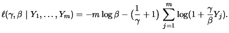
Definition 18.9 (POT Estimator)
The
POT estimator

for the
exceedance probability

for large
, is
whereby

are suitable estimators for

and

respectively.
can be, for example, calculated as
maximum likelihood estimators from the excesses
. First let's consider the case where
N is a
constant and where
is a
constant and where
 is a sample of i.i.d. random
variables with the distribution
is a sample of i.i.d. random
variables with the distribution
 .
Thus
is literally a Pareto distribution and
has the probability density
.
Thus
is literally a Pareto distribution and
has the probability density
Therefore, the log likelihood function is
By maximizing this
function with respect to
we obtain the maximum
likelihood (ML) estimator
 Analogously
we could also define the ML estimator for the parameter of the
generalized Pareto distribution using
Analogously
we could also define the ML estimator for the parameter of the
generalized Pareto distribution using
 .
.
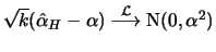
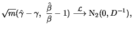
Theorem 18.7
For all

it holds for

with
i.e.

are asymptotically normally distributed.
In addition they are asymptotically efficient estimators.
In our initial problem
 N
N was random. Here the estimators
we just defined,
was random. Here the estimators
we just defined,
 and
and  are the
conditional ML estimators given
N
are the
conditional ML estimators given
N The asymptotic
distribution theory is also known in this case; in order to avoid
an asymptotic bias,
The asymptotic
distribution theory is also known in this case; in order to avoid
an asymptotic bias,
 must fulfill an additional
regularity condition. After we find an estimator for the
exceedance probability and thus a cdf for large , we
immediately obtain an estimator for the extreme quantile.
must fulfill an additional
regularity condition. After we find an estimator for the
exceedance probability and thus a cdf for large , we
immediately obtain an estimator for the extreme quantile.
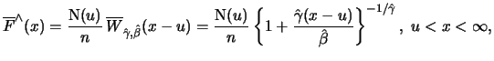
Definition 18.10 (POT Quantile Estimator)
The
POT Quantile estimator 
for the

-quantile

is the solution to
i.e.
SFEpotquantile.xpl
We can compare these estimators with the usual sample quantiles.
To do this we select a threshold value so that exactly
excesses lie beyond , that is
N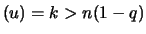 and thus
 . The POT quantile estimator that is
dependent on the choice of respectively is
where
. The POT quantile estimator that is
dependent on the choice of respectively is
where
 is the ML
estimator, dependent on the choice of , for and
. The corresponding sample quantile is
This is in approximate agreement with
is the ML
estimator, dependent on the choice of , for and
. The corresponding sample quantile is
This is in approximate agreement with
 when the
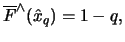
minimal value
when the
minimal value
![$ k=[n(1-q)] + 1$](sfehtmlimg3638.gif) is chosen for . Simulation
studies show that the value
is chosen for . Simulation
studies show that the value  of , which minimizes the mean
squared error
MSE
of , which minimizes the mean
squared error
MSE , is much larger than
![$ [n(1-q)] + 1$](sfehtmlimg3641.gif) , i.e., the POT
estimator for
, i.e., the POT
estimator for  differs distinctly from the sample quantile
 and is superior to it with respect to the mean
squared error when the threshold respectively is cleverly
chosen.
and is superior to it with respect to the mean
squared error when the threshold respectively is cleverly
chosen.
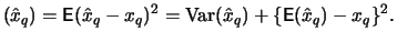
We are interested in a threshold , for which the mean squared
error of is as small as possible. The error can be
split up into the variance and the squared bias of :
MSE
- -
- when is too large, there are few
excesses
 N, and the estimator's variance is too
large,
N, and the estimator's variance is too
large,
- -
- when is too small, the approximation of the
excess distribution using a generalized Pareto distribution is not
good enough, and the bias
 is no longer
reliable.
is no longer
reliable.
An essential aid in selecting an appropriate threshold is the
average excess plot, which is approximately linear beyond the
appropriate threshold. This has already been discussed in Theorem
17.5, when one considers the relationship between the
Fréchet distribution as the asymptotic distribution of the
maxima and the Pareto distribution as the asymptotic distribution
of the excesses. It is supported by the following result for the
Pareto and exponential distributions
 .
.
Theorem 18.8
Let

be a
distributed random variable with

. The average excess function is linear:
With the usual
parametrization of the Pareto distribution

, i.e., the condition

means that
and thus

This result motivates the following application in choosing the
threshold: select the threshold of the POT estimator so that
the empirical average excess function  for values
  is approximately linear. An appropriate is chosen by
considering the average excess plots, where it is recommended that
the largest points
is approximately linear. An appropriate is chosen by
considering the average excess plots, where it is recommended that
the largest points
 along the righthand edge of the plot be excluded, since their
large variability for the most part distorts the optical
impression.
along the righthand edge of the plot be excluded, since their
large variability for the most part distorts the optical
impression.
The POT method for estimating the exceedance probability and the
extreme quantiles can be used on data with cdf that is in the MDA
of a Gumbel or a Fréchet distribution, as long as the expected
value is finite. Even for extreme financial data, this estimator
seems reasonable based on empirical evidence. A classic
alternative to the POT method is the Hill estimator, which was
already discussed in Chapter 12 in connection with the
estimation of the tail exponents of the DAX stocks. It is of
course only useful for distributions with slowly decaying tails,
such as those in the MDA of the Fréchet distribution, and
performs in simulations more often worse in comparison to the POT
estimator. The details are briefly introduced in this section.
In this section we will always assume that the data
 are i.i.d. with a distribution function in the MDA of
for some
are i.i.d. with a distribution function in the MDA of
for some
 . Due to Theorem 17.3 this is the case when
 with a slowly varying
function
with a slowly varying
function  . The tapering behavior of
 for increasing is mainly determined by the so called
tail exponents
for increasing is mainly determined by the so called
tail exponents  . The starting
point of the Hill method is the following estimator for .
. The starting
point of the Hill method is the following estimator for .
Definition 18.11 (Hill estimator)
are the order
statistics in decreasing order. The
Hill estimator

of the tail exponents
for a suitable

is
The form of the estimator can be seen from the following simple
special case. In general it holds that
 , but we now assume that with a fixed
 is constant. Set
 , it holds
that
, it holds
that
 are therefore
independent exponentially distributed random variables with
parameter . As is well known it holds that
are therefore
independent exponentially distributed random variables with
parameter . As is well known it holds that
 , and the ML estimator
 for is
 , where
 stands for the sample
average of
, thus,
where for the last equation only the
order of addition was changed.
is already similar
to the Hill estimator. In general it of course only holds that
stands for the sample
average of
, thus,
where for the last equation only the
order of addition was changed.
is already similar
to the Hill estimator. In general it of course only holds that
 for
sufficiently large . The argument for the special case is
similar for the largest observations
for
sufficiently large . The argument for the special case is
similar for the largest observations
 beyond the threshold , so that only
the largest order statistics enter the definition of the Hill
estimator.
beyond the threshold , so that only
the largest order statistics enter the definition of the Hill
estimator.
The Hill estimator is consistent, that is it converges in
probability to when
 such that
  . Under an additional condition it can also be shown that
 , i.e.,
is
asymptotically normally distributed.
, i.e.,
is
asymptotically normally distributed.
Similar to the POT estimator when considering the Hill estimator
the question regarding the choice of the threshold
 comes into play, since the observations located beyond it enter
the estimation. Once again we have a bias variance dilemma:
comes into play, since the observations located beyond it enter
the estimation. Once again we have a bias variance dilemma:
- -
- When is too small, only a few observations
influence
, and the variance of the estimator,
which is
 asymptotically, is too large,
- -
- when
is too large, the assumption underlying the derivation of the
estimator, i.e., that
 is approximately constant for all
 , is in general not well met and the bias
 becomes too large.
Based on the fundamentals of the Hill estimator for the tail
exponents we obtain direct estimators for the exceedance
probability
and for the quantiles of . Since
with a slowly varying
function , it holds for large
that:
 |
(18.5) |
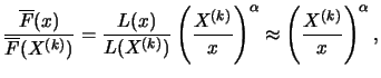
Because exactly one portion  of the data is larger
or equal to the order statistic
of the data is larger
or equal to the order statistic  , this is the
  sample quantile. Therefore, the empirical distribution function
takes on the value
sample quantile. Therefore, the empirical distribution function
takes on the value  at , since it uniformly
converges to the distribution function , for sufficiently large
at , since it uniformly
converges to the distribution function , for sufficiently large
 a that is not too large in comparison to
  yields:
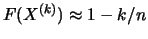 , i.e.,
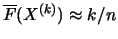 . Substituting this into (17.5), we obtain a Hill
esitmator for the exceedance probability
. Substituting this into (17.5), we obtain a Hill
esitmator for the exceedance probability
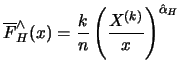
 By inverting this estimator we have the Hill quantile estimator for the
 quantile with

with
 , where the second
representation clearly shows the similarities and differences to
the POT quantile estimator.
, where the second
representation clearly shows the similarities and differences to
the POT quantile estimator.
SFEhillquantile.xpl
![\includegraphics[width=1\defpicwidth]{mexplot.ps}](sfehtmlimg3584.gif)
![$\displaystyle \hat{x}_q = u + \frac{\hat{\beta}}{\hat{\gamma}} \left[ \left\{ \frac{n}{\text{\rm N}(u)}
(1-q) \right\} ^ {-\hat{\gamma}} - 1 \right] . $](sfehtmlimg3631.gif)
![$\displaystyle \hat{x}_{q,k} = X^ {(k+1)} + \frac{\hat{\beta}_k}{\hat{\gamma}_k}
\left[ \left\{ \frac{n}{k} (1-q)\right\}^ {- \hat{\gamma}_k}
-1\right],$](sfehtmlimg3634.gif)
![$\displaystyle X^ {(k)} + X^ {(k)} \left[ \left\{ \frac{n}{k} (1-q) \right\}
^ {- \hat{\gamma}_H} - 1 \right]$](sfehtmlimg3696.gif)
![\includegraphics[width=1\defpicwidth]{jpyusd.ps}](sfehtmlimg3581.gif)
![\includegraphics[width=0.6\defpicwidth]{cdfp.ps}](sfehtmlimg3582.gif)
![\includegraphics[width=0.6\defpicwidth]{qa.ps}](sfehtmlimg3583.gif)