As was mentioned in the previous chapter,
the measures of goodness of fit are aimed at quantifying how well the
OLS regression we have obtained fits the data. The two measures
that are usually presented are the standard error of the
regression and the ![]() .
.
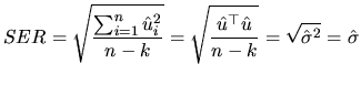
In the estimation section, we proved that if the regression model contains intercept, then the sum of the residuals are null (expression 2.32), so the average magnitude of the residuals can be expressed by its sample standard deviation, that is to say, by:

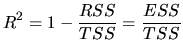
If we want to compare the goodness of fit between two models
whose endogenous variables are different, the ![]() is a more
adequate measure than the standard error of the regression,
because the
is a more
adequate measure than the standard error of the regression,
because the ![]() does not depend on the magnitude of the
variables. In order to obtain this measure, we begin, similarly
to the univariate linear model by writing the variance
decomposition expression, which divides the sample total
variation (TSS) in
does not depend on the magnitude of the
variables. In order to obtain this measure, we begin, similarly
to the univariate linear model by writing the variance
decomposition expression, which divides the sample total
variation (TSS) in ![]() , into the variation which is explained by
the model, or explained sum of squares (ESS), and the variation
which is not explained by the model, or residual sum of squares (RSS):
, into the variation which is explained by
the model, or explained sum of squares (ESS), and the variation
which is not explained by the model, or residual sum of squares (RSS):
From (2.129) we can deduce that, if the regression
explains all the total variation in ![]() , then
, then ![]() , which
implies
, which
implies ![]() . However, if the regression explains nothing,
then
. However, if the regression explains nothing,
then ![]() and
and ![]() . Thus, we can conclude that
. Thus, we can conclude that ![]() is
bounded between 0 and 1, in such a way that values of it close
to one imply a good fit of the regression.
is
bounded between 0 and 1, in such a way that values of it close
to one imply a good fit of the regression.
Nevertheless, we should be careful in forming conclusions, because
the magnitude of the ![]() is affected by the kind of data
employed in the model. In this sense, when we use time series data
and the trends of the endogenous and the explanatory variables are
similar, then the
is affected by the kind of data
employed in the model. In this sense, when we use time series data
and the trends of the endogenous and the explanatory variables are
similar, then the ![]() is usually large, even if there is no
strong relationship between these variables. However, when we work
with cross-section data , the
is usually large, even if there is no
strong relationship between these variables. However, when we work
with cross-section data , the ![]() tends to be lower, because
there is no trend, and also due to the substantial natural
variation in individual behavior. These arguments usually lead the
researcher to require a higher value of this measure if the
regression is carried out with time series data.
tends to be lower, because
there is no trend, and also due to the substantial natural
variation in individual behavior. These arguments usually lead the
researcher to require a higher value of this measure if the
regression is carried out with time series data.
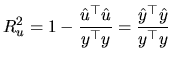
The bounds of the ![]() we have mentioned do not hold when the
estimated model does not contain an intercept. As
Patterson (2000) shows, this measure can be larger than one,
and even negative. In such cases, we should use an
we have mentioned do not hold when the
estimated model does not contain an intercept. As
Patterson (2000) shows, this measure can be larger than one,
and even negative. In such cases, we should use an
![]()
![]() as a measure of fit, which is
constructed in a similar way as the
as a measure of fit, which is
constructed in a similar way as the ![]() , but where neither
, but where neither
![]() nor
nor ![]() are calculated by using the variables in
deviations, that is to say:
are calculated by using the variables in
deviations, that is to say:
In practice, very often several regressions are estimated with
the same endogenous variable, and then we want to compare them
according to their goodness of fit. For this end, the ![]() is
not valid, because it never decreases when we add a new
explanatory variable. This is due to the mathematical properties
of the optimization which underly the LS procedure. In this sense,
when we increase the number of regressors, the objective function
is
not valid, because it never decreases when we add a new
explanatory variable. This is due to the mathematical properties
of the optimization which underly the LS procedure. In this sense,
when we increase the number of regressors, the objective function
![]() decreases or stays the same, but never
increases. Using (2.130), we can improve the
decreases or stays the same, but never
increases. Using (2.130), we can improve the ![]() by
adding variables to the regression, even if the new regressors do
not explain anything about
by
adding variables to the regression, even if the new regressors do
not explain anything about ![]() .
.
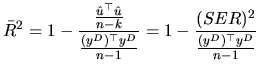
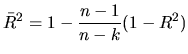
In order to avoid this behavior, we compute the so-called
adjusted ![]()
![]() as:
as:
Given that ![]() does not vary when we add a new regressor, we
must focus on the numerator of (2.132). When a new
variable is added to the set of regressors, then
does not vary when we add a new regressor, we
must focus on the numerator of (2.132). When a new
variable is added to the set of regressors, then ![]() increases,
and both
increases,
and both ![]() and
and
![]() decrease, so we must
find out how fast each of them decrease. If the decrease of
decrease, so we must
find out how fast each of them decrease. If the decrease of ![]() is less than that of
is less than that of
![]() , then
, then
![]() increases, while it decreases if the reduction of
increases, while it decreases if the reduction of
![]() is less than that of
is less than that of ![]() . The
. The ![]() and
and
![]() are usually presented in the softwar.
are usually presented in the softwar.
The relationship between ![]() and
and
![]() is given by:
is given by:
With respect to the ![]() , there is an inverse relationship
between it and
, there is an inverse relationship
between it and
![]() : if
: if ![]() increases, then
increases, then
![]() decreases, and vice versa.
decreases, and vice versa.
Finally, we should note that these measures should not be used if
we are comparing regressions which have a different endogenous
variable, even if they are based on the same set of data (for
example, ![]() and
and ![]() ). Moreover, when we want to evaluate an
estimated model, other statistics, together with these measures of
fit, must be calculated. These usually refer to the maintenance of
the classical assumptions of the MLRM.
). Moreover, when we want to evaluate an
estimated model, other statistics, together with these measures of
fit, must be calculated. These usually refer to the maintenance of
the classical assumptions of the MLRM.