In this section we consider the problem of recovering the regression function from noisy data based on a wavelet decomposition.
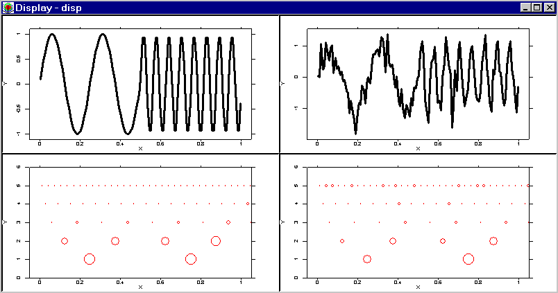
The upper two plots in the display show the underlying regression function (left) and noisy data (right). The lower two plots show the distribution of the wavelet coefficients in the time-scale domain for the regression function and the noisy data.
For simplicity we deal with a regression estimation problem. The noise is assumed to be additive and Gaussian with zero mean and unknown variance. Since the wavelet transform is an orthogonal transform we can consider the filtering problem in the space of wavelet coefficients. One takes the wavelet transform of the noisy data and tries to estimate the wavelet coefficients. Once the estimator is obtained one takes the inverse wavelet transform and recovers the unknown regression function.
To suppress the noise in the data two approaches are normally used. The first one is the so-called linear method. We have seen in Section 14.6 that the wavelet decomposition reflects well the properties of the signal in the frequency domain. Roughly speaking, higher decomposition scales correspond to higher frequency components in the regression function. If we assume that the underlying regression is allocated in the low frequency domain then the filtering procedure becomes evident. All empirical wavelet coefficients beyond some resolution scale are estimated by zero. This procedure works well if the signal is sufficiently smooth and when there is no boundary effect in the data. But for many practical problems such an approach does not seem to be fully appropriate, e.g. images cannot be considered as smooth functions.
To avoid this shortcoming often a nonlinear filtering procedure is used to suppress the noise in the empirical wavelet coefficients. The main idea is based on the fundamental property of the wavelet transform: father and mother functions are well localized in time domain. Therefore one could estimate the empirical wavelet coefficients independently. To do this let us compare the absolute value of the empirical wavelet coefficient and the standard deviation of the noise. It is clear that if the wavelet coefficient is of the same order of the noise level, then we cannot separate the signal and the noise. In this situation a good estimator for the wavelet coefficient is zero. In the case when an empirical wavelet coefficient is greater than the noise level a natural estimator for a wavelet coefficient is the empirical wavelet coefficient itself. This idea is called thresholding.
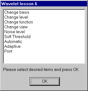
We divide the different modifications of thresholding in mainly three methods: hard thresholding, soft thresholding and a levelwise thresholding using Stein risk estimator, see Subsection 14.7.3.
To suppress the noise we apply the following nonlinear transform to
the empirical wavelet coefficients:
![]() ,
where
,
where ![]() is a certain threshold. The choice of the threshold is a
very delicate and important statistical problem.
is a certain threshold. The choice of the threshold is a
very delicate and important statistical problem.
On the one hand, a big threshold leads to a large bias of the estimator. But on the other hand, a small threshold increases the variance of the smoother. Theoretical considerations yield the following value of the threshold:
We provide two possibilities for choosing a threshold. First of all
you can do it by ``eye'' using the Hard threshold item and
entering the desired value of the threshold. The threshold offered is
the one described in the paragraph before. Note that this threshold
value is in most cases conservative and therefore we should choose a
threshold value below the offered one. The item Automatic
means that the threshold will be chosen as
![]() with a suitably estimated variance.
with a suitably estimated variance.
The plots of the underlying regression function and the data corrupted by the noise are shown in top of the display. You can change the variance of the noise and the regression function by using the Noise level and the Change function items.
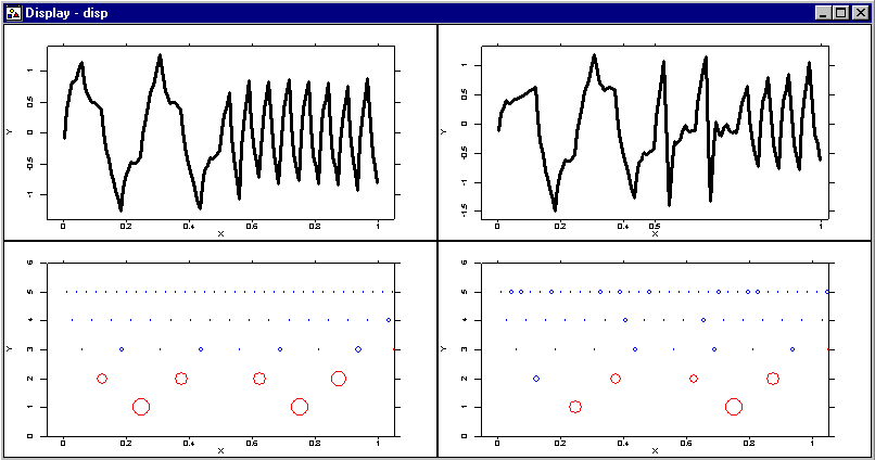
On the display above you can see the estimated regression function after the thresholding procedure. The left upper window shows how the threshold procedure distorts the underlying regression function when there is no noise in the data. The final estimator is shown in the right upper window.
Two plots in the bottom of the display show the thresholded and the nonthresholded wavelet coefficients. The thresholded coefficients are shown as blue circles and the nonthresholded as red ones. The radii of the circles correspond to the magnitudes of the empirical wavelet coefficients.
You can try to improve the estimator using the items Change basis and Change level. Under an appropriate choice of the parameters you can decrease the bias of your smoother.
Along with hard thresholding in many statistical applications soft thresholding procedures are often used. In this section, we study the so-called wavelet shrinkage procedure for recovering the regression function from noisy data.
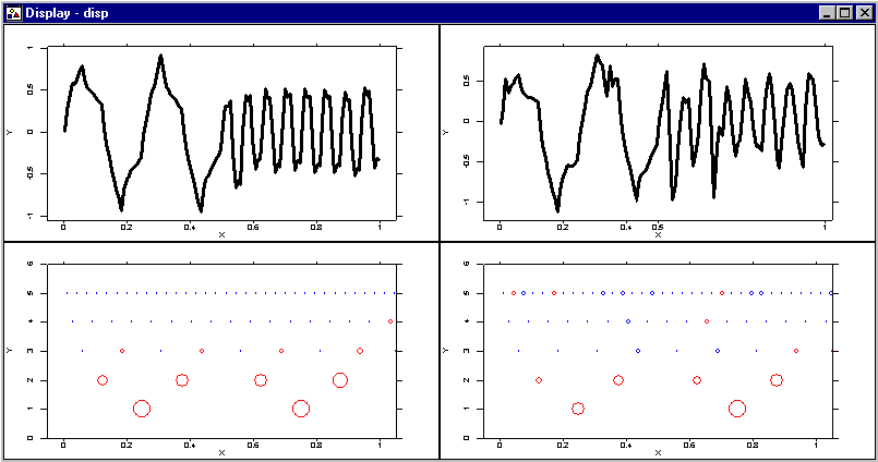
The display shows the same regression function as in the lesson before, without and with noise, after soft thresholding.
The only difference between the hard and the soft thresholding procedures is in the choice of the nonlinear transform on the empirical wavelet coefficients. For soft thresholding the following nonlinear transform is used:
In addition you can use a data driven procedure for choosing the
threshold. This procedure is based on Stein's principle of unbiased
risk estimation (Donoho and Johnstone; 1995). The main idea of this
procedure is the following. Since ![]() is a continuous function,
given
is a continuous function,
given ![]() , one can obtain an unbiased risk estimate for the soft
thresholding procedure. Then the optimal threshold is obtained by
minimization of the estimated risks.
, one can obtain an unbiased risk estimate for the soft
thresholding procedure. Then the optimal threshold is obtained by
minimization of the estimated risks.
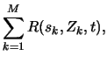
We first give an intuitive idea about adaptive thresholding using Stein's principle. Later on we give a detailed mathematical description of the procedure.
We define a risk function
![]() with
with
![]() , where
, where ![]() is the unknown coefficient,
is the unknown coefficient, ![]() known (or to be estimated) scale parameters,
known (or to be estimated) scale parameters, ![]() i.i.d.
i.i.d. ![]() random variables and
random variables and ![]() the threshold.
the threshold.
Since Stein enables us to estimate the risk
This procedure can be performed for each resolution level.
Mathematical derivation
Now we discuss the data driven choice of threshold,
initial level ![]() and the wavelet basis by the Stein (1981)
method of unbiased risk estimation. The argument below follows
Donoho and Johnstone (1995).
and the wavelet basis by the Stein (1981)
method of unbiased risk estimation. The argument below follows
Donoho and Johnstone (1995).
We first explain the Stein method for the idealized one-level
observation model discussed in the previous section:
![]() , for
, for
![]() ,
where
,
where
![]() is the vector of unknown parameters,
is the vector of unknown parameters,
![]() are known scale parameters and
are known scale parameters and ![]() are i.i.d.
are i.i.d. ![]() random variables.
random variables.
Let
![]() be an estimator of
be an estimator of ![]() . Introduce the
mean squared risk of the estimate of
. Introduce the
mean squared risk of the estimate of ![]() :
:
![]() .
.
Assume that the estimators ![]() have the form
have the form
If the true parameters ![]() were known, one could compute
were known, one could compute ![]() explicitly. In practice this is not possible, and one chooses a certain
approximation
explicitly. In practice this is not possible, and one chooses a certain
approximation ![]() of
of ![]() as a minimizer of an unbiased estimator
as a minimizer of an unbiased estimator ![]() of the risk
of the risk ![]() . To construct
. To construct ![]() , note that
, note that
| (14.3) |
The Stein principle is to minimize ![]() with respect to
with respect to ![]() and take the
minimizer
and take the
minimizer
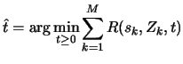 |
(14.4) |
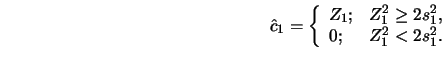
In the rest of this paragraph we formulate the Stein principle for the example of soft thresholding wavelet estimators. For soft thresholding (see above) we have
An equivalent expression is
The expression in square brackets in (14.5) does not depend on ![]() .
Thus, the definition (14.2) is equivalent to
.
Thus, the definition (14.2) is equivalent to
Let
![]() be the permutation ordering the array
such that
be the permutation ordering the array
such that ![]() ,
,
![]() :
:
![]() and
and
![]() . According to (14.6) one obtains
. According to (14.6) one obtains
![]() where
where
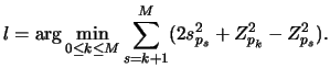
In particular for ![]() the above equation yields the following
estimator
the above equation yields the following
estimator
It is easy to see that the computation of the estimate of ![]() defined
above requires approximately
defined
above requires approximately ![]() operations provided that a
quick sort algorithm is used to order the array
operations provided that a
quick sort algorithm is used to order the array ![]() ,
,
![]() .
.
We proceed from the idealized model
![]() to a
more realistic density estimation model. In the context of wavelet
smoothing the principle of unbiased risk estimation gives the
following possibilities for adaptation:
to a
more realistic density estimation model. In the context of wavelet
smoothing the principle of unbiased risk estimation gives the
following possibilities for adaptation:
Please notice that in XploRe we have implemented the first version. To demonstrate these possibilities consider the family of wavelet estimators
![$\displaystyle \hat{R}(t,j_0,\varphi)=\sum_kR(s_{j_0 k}[\varphi],\hat{\alpha}_{j_0 k},t)+
\sum_{j=j_0}^{j_1}\sum_kR(s_{jk}[\psi],\hat{\beta}_{jk},t_j),
$](xlghtmlimg1885.gif)
In the third case we assume that the minimum is taken over a finite number of given wavelet bases.
Remark 1:
Since in practice the values of the different variances are not
available, one can use their empirical versions instead. For example
if (14.7) is the wavelet density estimator based on the sample
![]() , one can replace
, one can replace
![]() by its estimator.
by its estimator.
It is clear that this yields a consistent estimator for the variances
under rather general assumptions on the basis functions and on the
underlying density of the ![]() 's.
's.
Remark 2:
If one wants to threshold only the coefficients
![]() ,
which is usually the
case, the function
,
which is usually the
case, the function ![]() for
for
![]() should be
identically zero. Therefore,
should be
identically zero. Therefore,
![]() should be replaced by
should be replaced by
![]() and Steins unbiased risk
estimator takes the form
and Steins unbiased risk
estimator takes the form
![$\displaystyle \hat{R}((t_{j_0},\dots,t_{j_1}),j_0,\varphi)=
\sum_k s^2_{jk}[\varphi]+\sum_{j=j_0}^{j_1}\sum_k R\left(s_{jk}[\psi],
\hat{\beta}_{jk},t_j\right).$](xlghtmlimg1897.gif)
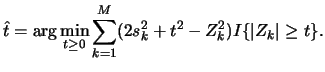
Let us now apply the Stein principle to a regression estimation
example. We choose the following step function for ![]() :
:
The function was observed at 128 equispaced points and disturbed
with Gaussian noise with variance ![]() . We use the Stein rule only
for threshold choice 1 (level by level) and not for the cases 2 and 3
where the adaptive choice of
. We use the Stein rule only
for threshold choice 1 (level by level) and not for the cases 2 and 3
where the adaptive choice of ![]() and of the basis is considered.
We thus choose the threshold
and of the basis is considered.
We thus choose the threshold ![]() as the minimizer with respect to
as the minimizer with respect to
![]() of
of
![$\displaystyle \hat{R}(t)=\sum_{j=j_0}^{j_1}\sum_k R\left(\hat{s}_{jk}[\psi],\hat{\beta}_{jk},
t_j\right),
$](xlghtmlimg1901.gif)
![$\displaystyle f^*(x,t,j_0,\psi)=\sum_k\alpha^*_{j_0 k}[\varphi,t]\varphi_{j_0 k}(x)+ \sum_{j=j_0}^{j_1}\sum_k \beta^*_{jk}[\psi,t_j]\psi_{jk}(x),$](xlghtmlimg1879.gif)