Next: 1.6 Impact of Heteroscedasticity
Up: 1. Model Selection
Previous: 1.4 Cross-Validation and Generalized
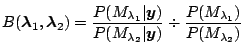
1.5 Bayes Factor
Let
 be the prior probability for model
 . For any two models
 and
and
 , the Bayes factor
 |
(1.29) |
is the posterior odds in favor of model
divided by the prior odds in favor of model
([31]). The Bayes factor provides a scale of
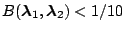
evidence in favor of one model versus another. For example,
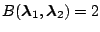 indicates that the data favor
model
over model
at odds of
two to one. Table 1.1 lists a possible
interpretation for Bayes factor suggested by
[29].
indicates that the data favor
model
over model
at odds of
two to one. Table 1.1 lists a possible
interpretation for Bayes factor suggested by
[29].
Table 1.1:
Jeffreys' scale of evidence for Bayes factors
| Bayes factor |
Interpretation |
 |
Strong evidence for
|
 |
Moderate evidence for
|
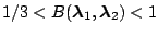 |
Weak evidence for
|
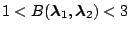 |
Weak evidence for
|
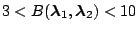 |
Moderate evidence for
|
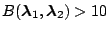 |
Strong evidence for
|
The Bayes factor is easy to understand and applicable to
a wide range of problems. Methods based on the Bayes factor
behave like an Occam's razor ([30]). Non-Bayesian analysis
typically selects a model and then proceeds as if the data is
generated by the chosen model. Ignoring the fact that the
model has been selected from the same data, this approach
often leads to under-estimation of the uncertainty in
quantities of interest, a problem know as the model
selection bias ([11]). Specifically, the
estimates of parameters based on the selected model are biased
and their variances are usually too optimistic. The Bayesian
approach accounts for model uncertainty with the posterior
probability
 . For example, to predict
a new observation
. For example, to predict
a new observation  , the best prediction under squared
loss is
, the best prediction under squared
loss is
a weighted average of predictions from all models with weights
equal to the posterior probabilities. Instead of using
a single model, such model averaging incorporates model
uncertainty. It also indicates that selecting a single model
may not be desirable or necessary for some applications such
as prediction ([27]).
The practical implementation of Bayesian model selection is,
however, far from straightforward. In order to compute the
Bayes factor (1.29), ones needs to specify priors
 as well as priors for parameters in each
model. While providing a way to incorporating other
information into the model and model selection, these priors
may be hard to set in practice, and standard non-informative
priors for parameters cannot be used
([6,18]). See [31],
[12] and [7] for more discussions on the
choice of priors.
as well as priors for parameters in each
model. While providing a way to incorporating other
information into the model and model selection, these priors
may be hard to set in practice, and standard non-informative
priors for parameters cannot be used
([6,18]). See [31],
[12] and [7] for more discussions on the
choice of priors.
After deciding on priors, one needs to
compute (1.29) which can be re-expressed as
 |
(1.30) |
where
 is the marginal likelihood. The
marginal likelihood usually involves an integral which can be
evaluated analytically only for some special cases. When the marginal
likelihood does not have a closed form, several methods for
approximation are available including Laplace approximation,
importance sampling, Gaussian quadrature and Markov chain Monte Carlo
(MCMC)
simulations.
Details about these methods are out of the scope of this chapter.
References can be found in [31].
is the marginal likelihood. The
marginal likelihood usually involves an integral which can be
evaluated analytically only for some special cases. When the marginal
likelihood does not have a closed form, several methods for
approximation are available including Laplace approximation,
importance sampling, Gaussian quadrature and Markov chain Monte Carlo
(MCMC)
simulations.
Details about these methods are out of the scope of this chapter.
References can be found in [31].
Under certain conditions, [32] showed that
Thus the
 is an approximation to the Bayes factor.
In the following we discuss selection of the smoothing
parameter
 for the
periodic spline. Based on (1.30), our goal is to
find
which maximizes the marginal likelihood
, or equivalently,
for the
periodic spline. Based on (1.30), our goal is to
find
which maximizes the marginal likelihood
, or equivalently,
 where
where
 is
the discrete Fourier transformation of
is
the discrete Fourier transformation of
 . Note that
 |
(1.31) |
where
 . Let
. Let
 . Assume
the following prior for
. Assume
the following prior for
 :
:
where  are mutually independent and are independent
of
are mutually independent and are independent
of
 . An improper prior is assumed for
 . It is not difficult to check that
 . Thus
the posterior means of the Bayes model (1.31)
and (1.32) are the same as the periodic spline
estimates.
. Thus
the posterior means of the Bayes model (1.31)
and (1.32) are the same as the periodic spline
estimates.
Let
 and
write
and
write
 . Since
 is
independent of
is
independent of  , we will estimate using the
marginal likelihood
, we will estimate using the
marginal likelihood
 . Since
 or
or
 , the log marginal likelihood of
 is
is
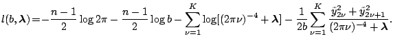
Fixing
and maximizing with respect to  , we have
Plugging back, we have
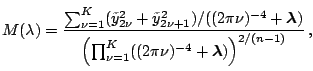
Thus maximizing the log likelihood is equivalent to minimizing
It is not difficult to check that
 |
(1.33) |
where
 is the product of non-zero eigenvalues.
The criterion (1.33) is called the
generalized maximum likelihood method in smoothing
spline literature ([50]). It is the same as the
restricted maximum likelihood (REML)
method in the mixed
effects literature ([53]). Note that the marginal
likelihood is approximated by plugging-in
is the product of non-zero eigenvalues.
The criterion (1.33) is called the
generalized maximum likelihood method in smoothing
spline literature ([50]). It is the same as the
restricted maximum likelihood (REML)
method in the mixed
effects literature ([53]). Note that the marginal
likelihood is approximated by plugging-in
 rather
than averaging over a prior distribution for .
rather
than averaging over a prior distribution for .
For the climate data, the GML scores for the periodic spline
and the corresponding fits are plotted in the left and right
panels of Fig. 1.7 respectively. The fits with
three different choices of the smoothing parameter are very
similar.
Next: 1.6 Impact of Heteroscedasticity
Up: 1. Model Selection
Previous: 1.4 Cross-Validation and Generalized
![$\displaystyle \notag l(\,\widehat{b},\boldsymbol{\lambda}) = \mathrm{constant} ...
...}} - \sum_{\nu=1}^K \log \left[ (2\pi \nu)^{-4}+\boldsymbol{\lambda} \right]\,.$](img3521.gif)