I start with the simplest metamodel, namely a first-order polynomial
with a single factor. An example is the 'Student' simulation in
Sect. 3.2, where I now assume that we are interested only in
the power so ![]() in (3.4) now denotes the type II error
predicted through the regression model. I further assume a single
factor (say)
in (3.4) now denotes the type II error
predicted through the regression model. I further assume a single
factor (say)
![]() ('relative' variability; i.e.,
absolute variability corrected for sample size); see
(3.4). Elementary mathematics proves that - to fit a straight
line - it suffices to have two input/output observations; see
'local area 1' in Fig. 3.1. It is simple to prove that the
'best' estimators of the regression parameters in (3.4)
result if those two values are as far apart as 'possible'.
('relative' variability; i.e.,
absolute variability corrected for sample size); see
(3.4). Elementary mathematics proves that - to fit a straight
line - it suffices to have two input/output observations; see
'local area 1' in Fig. 3.1. It is simple to prove that the
'best' estimators of the regression parameters in (3.4)
result if those two values are as far apart as 'possible'.
![\includegraphics[clip]{text/3-3/fig1.eps}](img3811.gif)
|
In practice, the analysts do not know over which experimental area a first-order polynomial is a 'valid' model. This validity depends on the goals of the simulation study; see Kleijnen and Sargent (2000).
So the analysts may start with a local area, and simulate the
two (locally) extreme input values. Let's denote these two extreme
values of the 'coded' variable ![]() by
by ![]() and
and ![]() , which
implies the following standardization of the original
variable
, which
implies the following standardization of the original
variable ![]() :
:
The Taylor series argument implies that - as the experimental area gets bigger (see 'local area 2' in Fig. 3.1) - a better metamodel may be a second-order polynomial:
I emphasize that the second-order polynomial in (3.6) is
nonlinear in ![]() (the regression variable), but linear in
(the regression variable), but linear in
![]() (the regression parameters or factor effects to be
estimated ). Consequently, such a polynomial is a type of
linear regression model (also see
Chap. II.8).
(the regression parameters or factor effects to be
estimated ). Consequently, such a polynomial is a type of
linear regression model (also see
Chap. II.8).
Finally, when the experimental area covers the whole area in which the simulation model is valid (see again Fig. 3.1), then other global metamodels become relevant. For example, Kleijnen and Van Beers (2003a) find that Kriging (discussed in Sect. 3.5) outperforms second-order polynomial fitting.
Note that Zeigler, Praehofer, and Kim (2000) call the experimental area the 'experimental frame'. I call it the domain of admissible scenarios, given the goals of the simulation study.
I conclude that lessons learned from the simple example in Fig. 3.1, are:
| Scenario |
|
|
|
|
| 0 | 0 | 0 | ||
| 0 | 0 | |||
| 0 | 0 |
Let's now consider a regression model with ![]() factors; for example,
factors; for example,
![]() . The design that is still most popular - even though it is
inferior - changes one factor at a time. For
. The design that is still most popular - even though it is
inferior - changes one factor at a time. For![]() such
a design is shown in Fig. 3.2 and Table 3.1; in this
table the factor values over the various factor combinations are shown
in the columns denoted by
such
a design is shown in Fig. 3.2 and Table 3.1; in this
table the factor values over the various factor combinations are shown
in the columns denoted by
![]() and
and
![]() ; the 'dummy'
column
; the 'dummy'
column
![]() corresponds with the polynomial intercept
corresponds with the polynomial intercept
![]() in (3.4). In this design the analysts
usually start with the 'base' scenario, denoted by the factor
combination
in (3.4). In this design the analysts
usually start with the 'base' scenario, denoted by the factor
combination ![]() ; see scenario 1 in the table. Next they run the two
scenarios
; see scenario 1 in the table. Next they run the two
scenarios ![]() and
and ![]() ; see the scenarios 2 and 3 in the table..
; see the scenarios 2 and 3 in the table..
In a one-factor-at-a-time design, the analysts cannot estimate the
interaction between the two factors. Indeed,
Table 3.1 shows that the estimated interaction (say)
![]() is confounded with the estimated intercept
is confounded with the estimated intercept
![]() ; i.e., the columns for the corresponding
regression variables are linearly dependent. (Confounding remains when
the base values are denoted not by zero but by one; then these two
columns become identical.)
; i.e., the columns for the corresponding
regression variables are linearly dependent. (Confounding remains when
the base values are denoted not by zero but by one; then these two
columns become identical.)
In practice, analysts often study each factor at three levels
(which may be denoted by ![]() ,
,
![]() ,
, ![]() ) in their one-at-a-time
design. However, two levels suffice to estimate the parameters of
a first-order polynomial (see again Sect. 3.4.1).
) in their one-at-a-time
design. However, two levels suffice to estimate the parameters of
a first-order polynomial (see again Sect. 3.4.1).
To enable the estimation of interactions, the analysts must change
factors simultaneously. An interesting problem arises if ![]() increases from two to three. Then Fig. 3.2 becomes
Fig. 3.3, which does not show the output (
increases from two to three. Then Fig. 3.2 becomes
Fig. 3.3, which does not show the output (![]() ), since it would
require a fourth dimension (instead
), since it would
require a fourth dimension (instead ![]() replaces
replaces ![]() ); the
asterisks are explained in Sect. 3.4.3. And Table 3.1
becomes Table 3.2. The latter table shows the
); the
asterisks are explained in Sect. 3.4.3. And Table 3.1
becomes Table 3.2. The latter table shows the ![]() factorial
design; i.e., in the experiment each of the three factors has two
values and all their combinations of values are simulated. To simplify
the notation, the table shows only the signs of the factor values, so
factorial
design; i.e., in the experiment each of the three factors has two
values and all their combinations of values are simulated. To simplify
the notation, the table shows only the signs of the factor values, so
![]() means
means ![]() and
and ![]() means
means ![]() . The table further shows possible
regression variables, using the symbols '0' through
'
. The table further shows possible
regression variables, using the symbols '0' through
'![]() ' - to denote the indexes of the regression variables
' - to denote the indexes of the regression variables
![]() (the dummy, always equal to
(the dummy, always equal to ![]() ) through
) through
![]() (third-order interaction). Further, I point out that each column is
balanced; i.e., each column has four plusses and four minuses
- except for the dummy column.
(third-order interaction). Further, I point out that each column is
balanced; i.e., each column has four plusses and four minuses
- except for the dummy column.
The ![]() design enables the estimation of all eight parameters of
the following regression model, which is a third-order polynomial that
is incomplete; i.e., some parameters are assumed zero:
design enables the estimation of all eight parameters of
the following regression model, which is a third-order polynomial that
is incomplete; i.e., some parameters are assumed zero:
Indeed, the ![]() design implies a matrix of regression
variables
design implies a matrix of regression
variables
![]() that is orthogonal:
that is orthogonal:
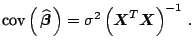
The covariance matrix of the (linear) OLS estimator given by (3.9) is
In case of white noise; i.e.,
However, I claim that in practice this white noise assumption does not hold:
Therefore I conclude that the analysts should choose between the following two options.
The variances of the estimated regression parameters - which are on
the main diagonal of
![]() in (3.10) - can be used to test statistically whether some
factors have zero effects. However, I emphasize that a significant
factor may be unimportant - practically speaking. If the factors are
scaled between
in (3.10) - can be used to test statistically whether some
factors have zero effects. However, I emphasize that a significant
factor may be unimportant - practically speaking. If the factors are
scaled between ![]() and
and ![]() (see the transformation in (3.5)),
then the estimated effects quantify the order of
importance. For example, in a first-order polynomial regression model
the factor estimated to be the most important factor is the one with
the highest absolute value for its estimated effect. See Bettonvil and
Kleijnen (1990).
(see the transformation in (3.5)),
then the estimated effects quantify the order of
importance. For example, in a first-order polynomial regression model
the factor estimated to be the most important factor is the one with
the highest absolute value for its estimated effect. See Bettonvil and
Kleijnen (1990).
The incomplete third-order polynomial in (3.7) included
a third-order effect, namely
![]() . Standard DOE
textbooks include the definition and estimation of such high-order
interactions. However, the following claims may be made:
. Standard DOE
textbooks include the definition and estimation of such high-order
interactions. However, the following claims may be made:
In this ![]() design two columns are identical, namely the
design two columns are identical, namely the
![]() column (with four plusses) and the dummy column. Hence, the
corresponding two effects are confounded - but the high-order
interaction
column (with four plusses) and the dummy column. Hence, the
corresponding two effects are confounded - but the high-order
interaction
![]() is assumed zero, so this confounding
can be ignored!
is assumed zero, so this confounding
can be ignored!
Sometimes a first-order polynomial suffices. For example, in
the (sequential) optimization of black-box simulation models the
analysts may use a first-order polynomial to estimate the local
gradient; see Angün et al. (2002). Then it suffices to take a
![]() design with the biggest
design with the biggest ![]() value that makes the
following condition hold:
value that makes the
following condition hold:
![]() . An example is:
. An example is: ![]() and
and
![]() so only
so only ![]() scenarios are simulated; see
Table 3.3. This table shows that the first three factors
(labeled
scenarios are simulated; see
Table 3.3. This table shows that the first three factors
(labeled ![]() ,
, ![]() , and
, and ![]() ) form a full factorial
) form a full factorial ![]() design; the
symbol '
design; the
symbol '![]() ' means that the values for factor
' means that the values for factor ![]() are
selected by multiplying the elements of the columns for the
factors
are
selected by multiplying the elements of the columns for the
factors ![]() and
and ![]() . Note that the design is still balanced and
orthogonal. Because of this orthogonality, it can be proven that the
estimators of the regression parameters have smaller variances than
one-factor-at-a-time designs give. How to select scenarios in
. Note that the design is still balanced and
orthogonal. Because of this orthogonality, it can be proven that the
estimators of the regression parameters have smaller variances than
one-factor-at-a-time designs give. How to select scenarios in ![]() designs is discussed in many DOE textbooks, including Kleijnen
(1975, 1987).
designs is discussed in many DOE textbooks, including Kleijnen
(1975, 1987).
Actually, these designs - i.e., fractional factorial designs of the
![]() type with biggest
type with biggest ![]() value still enabling the estimation
of first-order polynomial regression models - are a subset of
Plackett-Burman designs. The latter designs consists of
value still enabling the estimation
of first-order polynomial regression models - are a subset of
Plackett-Burman designs. The latter designs consists of ![]() combinations with
combinations with ![]() rounded upwards to a multiple of four;
for example, if
rounded upwards to a multiple of four;
for example, if ![]() , then Table 3.4 applies. If
, then Table 3.4 applies. If ![]() ,
then the Plackett-Burman design is a
,
then the Plackett-Burman design is a
![]() fractional factorial
design; see Kleijnen (1975, pp. 330-331). Plackett-Burman designs are
tabulated in many DOE textbooks, including Kleijnen (1975). Note that
designs for first-order polynomial regression models are called
resolution III designs.
fractional factorial
design; see Kleijnen (1975, pp. 330-331). Plackett-Burman designs are
tabulated in many DOE textbooks, including Kleijnen (1975). Note that
designs for first-order polynomial regression models are called
resolution III designs.
Resolution IV designs enable unbiased estimators of
first-order effects - even if two-factors interactions are
important. These designs require double the number of scenarios
required by resolution III designs; i.e., after simulating the
scenarios of the resolution III design, the analysts simulate the
mirror scenarios; i.e., multiply by ![]() the factor values in
the original scenarios.
the factor values in
the original scenarios.
Resolution V designs enable unbiased estimators of
first-order effects plus all two-factor interactions. To this class
belong certain ![]() designs with small enough
designs with small enough ![]() values. These
designs often require rather many scenarios to be
simulated. Fortunately, there are also saturated designs;
i.e., designs with the minimum number of scenarios that still allow
unbiased estimators of the regression parameters. Saturated designs
are attractive for expensive simulations; i.e., simulations
that require relatively much computer time per scenario. Saturated
resolution V designs were developed by Rechtschaffner (1967).
values. These
designs often require rather many scenarios to be
simulated. Fortunately, there are also saturated designs;
i.e., designs with the minimum number of scenarios that still allow
unbiased estimators of the regression parameters. Saturated designs
are attractive for expensive simulations; i.e., simulations
that require relatively much computer time per scenario. Saturated
resolution V designs were developed by Rechtschaffner (1967).
Central composite designs (CCD) are meant for the estimation
of second-order polynomials. These designs augment resolution V
designs with the base scenario and ![]() scenarios that change factors
one at a time; this changing increases and decreases each factor in
turn. Saturated variants (smaller than CCD) are discussed in Kleijnen
(1987, pp. 314-316).
scenarios that change factors
one at a time; this changing increases and decreases each factor in
turn. Saturated variants (smaller than CCD) are discussed in Kleijnen
(1987, pp. 314-316).
The main conclusion is that incomplete designs for low-order polynomial regression are plentiful in both the classic DOE literature and the simulation literature. (The designs in the remainder of this chapter are more challenging.)
Most practical, non-academic simulation models have many factors; for
example, Kleijnen et al. (2003b) experiment with a supply-chain
simulation model with nearly
![]() factors. Even
a Plackett-Burman design would then take
factors. Even
a Plackett-Burman design would then take
![]() scenarios. Because each scenario needs to be replicated
several times, the total computer time may then be prohibitive. For
that reason, many analysts keep a lot of factors fixed (at their base
values), and experiment with only a few remaining factors. An example
is a military (agent-based) simulation that was run millions of times
for just a few scenarios - changing only a few factors; see Horne and
Leonardi (2001).
scenarios. Because each scenario needs to be replicated
several times, the total computer time may then be prohibitive. For
that reason, many analysts keep a lot of factors fixed (at their base
values), and experiment with only a few remaining factors. An example
is a military (agent-based) simulation that was run millions of times
for just a few scenarios - changing only a few factors; see Horne and
Leonardi (2001).
However, statisticians have developed designs that require fewer than
![]() scenarios - called supersaturated designs; see Yamada
and Lin (2002). Some designs aggregate the
scenarios - called supersaturated designs; see Yamada
and Lin (2002). Some designs aggregate the ![]() individual
factors into groups of factors. It may then happen that the effects of
individual factors cancel out, so the analysts would erroneously
conclude that all factors within that group are unimportant. The
solution is to define the
individual
factors into groups of factors. It may then happen that the effects of
individual factors cancel out, so the analysts would erroneously
conclude that all factors within that group are unimportant. The
solution is to define the ![]() and
and ![]() levels of the individual
factors such that all first-order effects
levels of the individual
factors such that all first-order effects
![]() (
(
![]() ) are non-negative. My experience is that in
practice the users do know the direction of the first-order effects of
individual factors.
) are non-negative. My experience is that in
practice the users do know the direction of the first-order effects of
individual factors.
There are several types of group screening designs; for a recent survey including references, I refer to Kleijnen et al. (2003b). Here I focus on the most efficient type, namely Sequential Bifurcation designs.
This design type is so efficient because it proceeds
sequentially. It starts with only two scenarios, namely, one
scenario with all individual factors at ![]() , and a second scenario
with all factors at
, and a second scenario
with all factors at ![]() . Comparing the outputs of these two extreme
scenarios requires only two replications because the aggregated effect
of the group factor is huge compared with the intrinsic noise (caused
by the pseudorandom numbers). The next step splits -
bifurcates - the factors into two groups. There are several
heuristic rules to decide on how to assign factors to groups (again
see Kleijnen et al. 2003b). Comparing the outputs of the third
scenario with the outputs of the preceding scenarios enables the
estimation of the aggregated effect of the individual factors within
a group. Groups - and all its individual factors - are eliminated
from further experimentation as soon as the group effect is
statistically unimportant. Obviously, the groups get smaller as the
analysts proceed sequentially. The analysts stop, once the first-order
effects
. Comparing the outputs of these two extreme
scenarios requires only two replications because the aggregated effect
of the group factor is huge compared with the intrinsic noise (caused
by the pseudorandom numbers). The next step splits -
bifurcates - the factors into two groups. There are several
heuristic rules to decide on how to assign factors to groups (again
see Kleijnen et al. 2003b). Comparing the outputs of the third
scenario with the outputs of the preceding scenarios enables the
estimation of the aggregated effect of the individual factors within
a group. Groups - and all its individual factors - are eliminated
from further experimentation as soon as the group effect is
statistically unimportant. Obviously, the groups get smaller as the
analysts proceed sequentially. The analysts stop, once the first-order
effects
![]() of all the important individual factors are
estimated. In their supply-chain simulation, Kleijnen et al. (2003b)
classify only
of all the important individual factors are
estimated. In their supply-chain simulation, Kleijnen et al. (2003b)
classify only ![]() of the
of the
![]() factors as important. (Next,
this shortlist of important factors is further investigated to find
a robust solution.)
factors as important. (Next,
this shortlist of important factors is further investigated to find
a robust solution.)
![\includegraphics[clip]{text/3-3/fig2.eps}](img3818.gif)
![\includegraphics[clip]{text/3-3/fig3.eps}](img3833.gif)
![$\displaystyle \boldsymbol{{\text{cov}}}(\,\boldsymbol{\widehat{\beta }}\,) = \l...
...ft(\boldsymbol{X}^{T}\boldsymbol{X}\right)^{-1}\boldsymbol{X}^{T}\right]^{T}\,.$](img3842.gif)