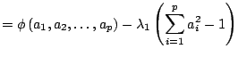
The ![]() -dimensional data can be reduced into
-dimensional data can be reduced into ![]() -dimensional data
using
-dimensional data
using ![]() linear combinations of
linear combinations of ![]() variables. The linear
combinations can be considered as linear projection. Most methods for
reduction involve the discovery of linear combinations of variables
under set criterion. Principal component analysis (PCA) and
projection pursuit are typical methods of this type. These methods
will be described in the following subsections.
variables. The linear
combinations can be considered as linear projection. Most methods for
reduction involve the discovery of linear combinations of variables
under set criterion. Principal component analysis (PCA) and
projection pursuit are typical methods of this type. These methods
will be described in the following subsections.
Suppose that we have observations of ![]() variables size
variables size ![]() ;
;
![]() (referred to as
(referred to as ![]() hereafter). PCA is conducted
for the purpose of constructing linear combinations of variables so
that their variances are large under certain conditions. A linear
combination of variables is denoted by
hereafter). PCA is conducted
for the purpose of constructing linear combinations of variables so
that their variances are large under certain conditions. A linear
combination of variables is denoted by
![]() (simply,
(simply,
![]() ), where
), where
![]() .
.
Then, the sample variance of
![]() can be represented by
can be represented by
 |
||
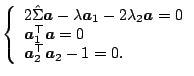
![$\displaystyle \left\{ \begin{array}{l}
2\hat{\Sigma}{\boldsymbol{a}}-2\lambda_...
...\ [1.5mm]
{\boldsymbol{a}}^{\top}{\boldsymbol{a}}-1=0{}.
\end{array}
\right.$](img4280.gif) |
The second principal components serve to explain the maximum variance
under the constraint and the fact that they are independent of the
first principal components. In other words, the second principal
components
![]() take the maximum variance under the
constraints
take the maximum variance under the
constraints
![]() and
and
![]() . The
second principal components can also be derived with Lagrange
multipliers;
. The
second principal components can also be derived with Lagrange
multipliers;
 |
We can obtain ![]() and
and ![]() is another eigenvalue (not
equal to
is another eigenvalue (not
equal to ![]() ). Since the variance of
). Since the variance of
![]() is
is
![]() , the
, the
![]() must be the second largest eigenvalue
of
must be the second largest eigenvalue
of
![]() .
.
![]() are
referred to as the second principal components. The third principal
components, fourth principal components,
are
referred to as the second principal components. The third principal
components, fourth principal components, ![]() , and the
, and the ![]() -th
principal components can then be derived in the same manner.
-th
principal components can then be derived in the same manner.
The first principal components through the ![]() -th principal components
were defined in the discussions above. As previously mentioned, the
variance of the
-th principal components
were defined in the discussions above. As previously mentioned, the
variance of the ![]() -th principal components is
-th principal components is ![]() . The sum of
variances of
. The sum of
variances of ![]() variables is
variables is
![]() , where
, where
![]() . It is well known that
. It is well known that
![]() ; the sum of the variances
coincides with the sum of the eigenvalues. The proportion
of the
; the sum of the variances
coincides with the sum of the eigenvalues. The proportion
of the ![]() -th principal components is defined as the proportion of the
entire variance to the variance of the
-th principal components is defined as the proportion of the
entire variance to the variance of the ![]() -th principal components:
-th principal components:
 |
 |
We have explained PCA as an eigenvalue problem of covariance matrix. However, the results of this method are affected by units of measurements or scale transformations of variables. Thus, another method is to employ a correlation matrix rather than a covariance matrix. This method is invariant under units of variables, but does not take the variances of the variables into account.
PCA searches a lower dimensional space that captures the majority of the variation within the data and discovers linear structures in the data. This method, however, is ineffective in analyzing nonlinear structures, i.e. curves, surfaces or clusters. In 1974, [2] proposed projection pursuit to search for linear projection onto the lower dimensional space that robustly reveals structures in the data. After that, many researchers developed new methods for projection pursuit and evaluated them (e.g. [6,1,4,7,17,10]). The fundamental idea behind projection pursuit is to search linear projection of the data onto a lower dimensional space their distribution is ''interesting''; ''interesting'' is defined as being ''far from the normal distribution'', i.e. the normal distribution is assumed to be the most uninteresting. The degree of ''far from the normal distribution'' is defined as being a projection index, the details of which will be described later.
The use of a projection index makes it possible to execute projection
pursuit with the projection index. Here is the fundamental algorithm
of ![]() -dimensional projection pursuit.
-dimensional projection pursuit.
The goal of projection pursuit is to find a projection that reveals interesting structures in the data. There are various standards for interestingness, and it is a very difficult task to define. Thus, the normal distribution is regarded as uninteresting, and uninterestingness is defined as a degree that is ''far from the normal distribution.''
Projection indexes are defined as of this degree. There are many definitions for projection indexes. Projection pursuit searches projections based on the projection index; methods of projection pursuit are defined by the projection indexes.
Here we will present several projection indexes. It is assumed that
![]() is the result of sphering
is the result of sphering
![]() ; the mean
vector is a zero vector and the covariance matrix is an identity
matrix.
; the mean
vector is a zero vector and the covariance matrix is an identity
matrix.
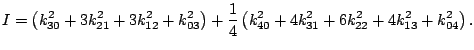
[1] proposed the following projection index:
In the case of two-dimensional projection pursuit, the index is represented by
![$\displaystyle = \sum_{j=1}^J(2j+1)E^2[P_j(R_1)]/4$](img4311.gif) |
||
![$\displaystyle \quad{} + \sum_{k=1}^J(2k+1)E^2\left[P_k(R_2)\right]/4$](img4312.gif) |
||
![$\displaystyle \quad{} + \sum_{j=1}^J\sum_{k=1}^{J-j}(2j+1)(2k+1)E^2\left[P_j(R_1)P_k(R_2)\right]/4{},$](img4313.gif) |
The third and higher cumulants of the normal distribution vanish. The
cumulants are sometimes used for the test of normality, i.e. they can
be used for the projection index. [8] proposed
a one-dimensional projection index named the ''moment index,'' with
the third cumulant
![]() and the fourth cumulant
and the fourth cumulant
![]() :
:
 |
For two-dimensional projection pursuit, the moment index can be defined as
 |
[4] proposed the following projection index:
![$\displaystyle I = \left[\theta_0({\boldsymbol{\alpha}})-2^{-1/2}\pi^{-1/4}\right]^2+\sum_{j=1}^J\theta_j^2({\boldsymbol{\alpha}}){},$](img4320.gif) |
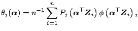 |
|
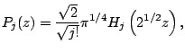 |
The main objective of ordinary projection pursuit is the discovery of non-normal structures in a dataset. Non-normality is evaluated using the degree of difference between the distribution of the projected dataset and the normal distribution.
There are times in which it is desired that special structures be discovered using criterion other than non-normal criterion. For example, if the purpose of analysis is to investigate a feature of a subset of the entire dataset, the projected direction should be searched so that the projected distribution of the subset is far from the distribution of the entire dataset. In sliced inverse regression (please refer to the final subsection of this chapter), the dataset is divided into several subsets based on the values of the response variable, and the effective dimension-reduction direction is searched for using projection pursuit. In this application of projection pursuit, projections for which the distributions of the projected subsets are far from those of the entire dataset are required. [16] proposed the adoption of relative projection pursuit for these purposes. Relative projection pursuit finds interesting low-dimensional space that differs from the reference dataset predefined by the user.
![$\displaystyle I = \frac{1}{2}\sum_{j=1}^J(2j+1)\left[ \frac{1}{n}\sum_{i=1}^nP_...
...ft({\boldsymbol{\alpha}}^{\top} {\boldsymbol{Z}}_i\right)-1\right) \right]^2{},$](img4307.gif)