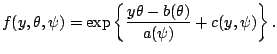
The generalized linear model is determined by two components:
We say that
a distribution is a member of the exponential family
if its probability mass function (if ![]() discrete) or its density
function (if
discrete) or its density
function (if ![]() continuous) has the following form:
continuous) has the following form:
| Range | Variance terms | ||||
| of |
|
||||
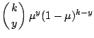
| Bernoulli
|
|
|
|
|
1 |
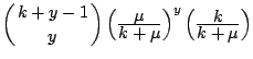
| Binomial
|
|
 |
|
|
1 |
| Poisson
|
|
|
|
1 | |
| Geometric
|
|
|
|
|
1 |
| Negative
Binomial
|
|
 |
|
 |
1 |
| Exponential
|
|
|
|
||
| Gamma
|
|
 |
|
|
|
| Normal
|
|
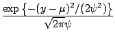 |
1 | ||
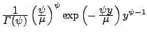
| Inverse
Gaussian |
|
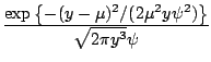 |
|
||
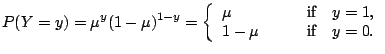
Table 7.1 lists some probability distributions that are
typically used for a GLM. For the binomial and negative
binomial distribution the additional parameter ![]() is assumed to be known.
Note also that the Bernoulli, geometric and
exponential distributions are special cases of the binomial, negative
binomial and Gamma distributions, respectively.
is assumed to be known.
Note also that the Bernoulli, geometric and
exponential distributions are special cases of the binomial, negative
binomial and Gamma distributions, respectively.
After
having specified the distribution of ![]() , the link function
, the link function ![]() is the second component to choose for the GLM. Recall the model
notation
is the second component to choose for the GLM. Recall the model
notation
![]() .
In the case that the canonical parameter
.
In the case that the canonical parameter ![]() equals
the linear predictor
equals
the linear predictor ![]() , i.e. if
, i.e. if
the link function is called the canonical link function. For models with a canonical link the estimation algorithm simplifies as we will see in Sect. 7.3.3. Table 7.2 shows in its second column the canonical link functions of the exponential family distributions presented in Table 7.1.
| Canonical link | Deviance | |
|
|
|
|
| Bernoulli
|
|
|
| Binomial
|
|
|
| Poisson
|
|
|
| Geometric
|
|
|
| Negative Binomial
|
|
![$ 2\sum \left[y_i\log\left(\frac{\displaystyle y_ik+y_i\mu_i}%
{\displaystyle \m...
...\left\{\frac{\displaystyle k(k+y_i)}%
{\displaystyle k(k+\mu_i)}\right\}\right]$](img4627.gif) |
| Exponential
|
|
|
| Gamma
|
|
|
| Normal
|
|
|
| Inverse
Gaussian |
|
![$ 2\sum \left[\frac{\displaystyle (y_i-\mu_i)^2}%
{\displaystyle y_i\mu_i^2}\right]$](img4632.gif) |
What link functions could we choose apart from the canonical?
For most of the models exists a number of specific link functions.
For Bernoulli ![]() , for example, any smooth
cdf can be used. Typical links
are the logistic and standard normal (Gaussian) cdfs
which lead to logit
and probit
models, respectively.
A further alternative for Bernoulli
, for example, any smooth
cdf can be used. Typical links
are the logistic and standard normal (Gaussian) cdfs
which lead to logit
and probit
models, respectively.
A further alternative for Bernoulli ![]() is the complementary log-log link
is the complementary log-log link
![]() .
.
A flexible class of link functions for positive ![]() observations
is the class of power functions. These links are given by
the Box-Cox transformation ([6]), i.e. by
observations
is the class of power functions. These links are given by
the Box-Cox transformation ([6]), i.e. by
![]() or
or
![]() where we
set in both cases
where we
set in both cases
![]() for
for ![]() .
.