Subsections

• 1.2.1 Characteristic Function Representation
• 1.2.2 Computation of Stable Density and Distribution Functions
• 1.2.3 Simulation of $\alpha$-stable Variables
• 1.2.4 Estimation of Parameters
  • 1.2.4.1 Sample Quantile Methods
  • 1.2.4.2 Sample Characteristic Function Methods
  • 1.2.4.3 Maximum Likelihood Method
  
  
• 1.2.5 Are Asset Returns $\alpha$-stable?
• 1.2.6 Truncated Stable Distributions

1.2 Stable Distributions

It is often argued that financial asset returns are the cumulative outcome of a vast number of pieces of information and individual decisions arriving almost continuously in time ([71,87]). As such, since the pioneering work of Louis Bachelier in 1900, they have been modeled by the Gaussian distribution. The strongest statistical argument for it is based on the Central Limit Theorem, which states that the sum of a large number of independent, identically distributed variables from a finite-variance distribution will tend to be normally distributed. However, financial asset returns usually have heavier tails.

In response to the empirical evidence [64] and [36] proposed the stable distribution as an alternative model. There are at least two good reasons for modeling financial variables using stable distributions. Firstly, they are supported by the generalized Central Limit Theorem, which states that stable laws are the only possible limit distributions for properly normalized and centered sums of independent, identically distributed random variables ([58]). Secondly, stable distributions are leptokurtic. Since they can accommodate the fat tails and asymmetry, they fit empirical distributions much better.

Stable laws - also called $\alpha$-stable, stable Paretian or Lévy stable - were introduced by [61] during his investigations of the behavior of sums of independent random variables. A sum of two independent random variables having an $\alpha$-stable distribution with index $\alpha$ is again $\alpha$-stable with the same index $\alpha$. This invariance property, however, does not hold for different $\alpha$'s.

Figure 1.3: A semilog plot of symmetric ( $\beta =\mu =0$) $\alpha$-stable probability density functions for $\alpha = 2$ (solid), $1.8$ (dotted), $1.5$ (dashed) and $1$ (long-dashed) showing the dependence on the tail exponent (left panel). The Gaussian ($\alpha = 2$) density forms a parabola and is the only $\alpha$-stable density with exponential tails. A plot of $\alpha$-stable probability density functions for $\alpha =1.2$ and $\beta = 0$ (solid), $0.5$ (dotted), $0.8$ (dashed) and $1$ (long-dashed) showing the dependence on the skewness parameter (right panel) (Q: STFstab01, STFstab02)

The $\alpha$-stable distribution requires four parameters for complete description: an index of stability $\alpha\in (0,2]$ also called the tail index, tail exponent or characteristic exponent, a skewness parameter $\beta\in [-1,1]$, a scale parameter $\sigma>0$ and a location parameter $\mu\in \mathbb{R}$. The tail exponent $\alpha$ determines the rate at which the tails of the distribution taper off, see the left panel of Fig. 1.3. When $\alpha = 2$, a Gaussian distribution results. When $\alpha<2$, the variance is infinite and the tails are asymptotically equivalent to a Pareto law, i.e. they exhibit a power-law behavior. More precisely, using a central limit theorem type argument it can be shown that ([48,90]):

$$\begin{cases}\lim_{x\rightarrow\infty} x^{\alpha} \mathbb{P}(... ...{P}(X<-x) = C_{\alpha}(1+\beta) \sigma^{\alpha}\;,& \end{cases}$$ (1.1)

where:

$$C_{\alpha}=\left(2\int_0^{\infty} x^{-\alpha} \sin(x) {\text{d}} x \right)^{-1} =\frac{1}{\pi}\Gamma(\alpha)\sin\frac{\pi\alpha}{2}\;.$$

When $\alpha>1$, the mean of the distribution exists and is equal to $\mu$. In general, the $p$th moment of a stable random variable is finite if and only if $p<\alpha$. When the skewness parameter $\beta$ is positive, the distribution is skewed to the right, i.e. the right tail is thicker, see the right panel of Fig. 1.3. When it is negative, it is skewed to the left. When $\beta = 0$, the distribution is symmetric about $\mu$. As $\alpha$ approaches $2$, $\beta$ loses its effect and the distribution approaches the Gaussian distribution regardless of $\beta$. The last two parameters, $\sigma$ and $\mu$, are the usual scale and location parameters, i.e. $\sigma$ determines the width and $\mu$ the shift of the mode (the peak) of the distribution.

1.2.1 Characteristic Function Representation

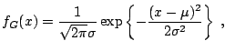
From a practitioner's point of view the crucial drawback of the stable distribution is that, with the exception of three special cases, its probability density function (PDF) and cumulative distribution function (CDF) do not have closed form expressions. These exceptions include the well known Gaussian ($\alpha = 2$) law, whose density function is given by:

$$f_G(x) = \frac{1}{\sqrt{2\pi}\sigma} \exp\left\{ -\frac{(x-\mu)^2}{2\sigma^2} \right\}\;,$$ (1.2)

and the lesser known Cauchy ($\alpha=1$, $\beta = 0$) and Lévy ( $\alpha =0.5$, $\beta=1$) laws.

Hence, the $\alpha$-stable distribution can be most conveniently described by its characteristic function $\phi(t)$ - the inverse Fourier transform of the PDF. However, there are multiple parameterizations for $\alpha$-stable laws and much confusion has been caused by these different representations. The variety of formulas is caused by a combination of historical evolution and the numerous problems that have been analyzed using specialized forms of the stable distributions. The most popular parameterization of the characteristic function of $X \sim S_{\alpha}(\sigma,\beta,\mu)$, i.e. an $\alpha$-stable random variable with parameters $\alpha$, $\sigma$, $\beta$ and $\mu$, is given by ([90,98]):

$$\log\phi(t) = \begin{cases}\displaystyle -\sigma^{\alpha}\vert t\... ...}(t)\frac{2}{\pi}\log\vert t\vert\right\}+ i \mu t\;, & \alpha=1\;. \end{cases}$$ (1.3)

Note, that the traditional scale parameter $\sigma$ of the Gaussian distribution is not the same as $\sigma$ in the above representation. A comparison of formulas (1.2) and (1.3) yields the relation: $\sigma_{\text{Gaussian}} = \sqrt{2} \sigma$.

Figure 1.4: Comparison of $S$ and $S^0$ parameterizations: $\alpha$-stable probability density functions for $\beta =0.5$ and $\alpha =0.5$ (solid), $0.75$ (dotted), $1$ (short-dashed), $1.25$ (dashed) and $1.5$ (long-dashed) (Q: STFstab04)

For numerical purposes, it is often useful to use Nolan's (1997) parameterization:

$$\log\phi_0(t) = \begin{cases}\displaystyle -\sigma^{\alpha}\vert ... ...}{\pi}\log(\sigma \vert t\vert)\right\}+ i \mu_0 t\;, & \alpha=1\;. \end{cases}$$ (1.4)

The $S^0_{\alpha}(\sigma,\beta,\mu_0)$ representation is a variant of Zolotarev's 1986 (M)-parameterization, with the characteristic function and hence the density and the distribution function jointly continuous in all four parameters, see Fig. 1.4. In particular, percentiles and convergence to the power-law tail vary in a continuous way as $\alpha$ and $\beta$ vary. The location parameters of the two representations are related by $\mu = \mu_0 - \beta\sigma\tan(\pi\alpha/2)$ for $\alpha\ne 1$ and $\mu = \mu_0 - \beta\sigma(2/\pi)\log\sigma$ for $\alpha=1$.

1.2.2 Computation of Stable Density and Distribution Functions

The lack of closed form formulas for most stable densities and distribution functions has negative consequences. Numerical approximation or direct numerical integration have to be used, leading to a drastic increase in computational time and loss of accuracy. Of all the attempts to be found in the literature a few are worth mentioning. [29] developed a procedure for approximating the stable distribution function using Bergström's (1952) series expansion. Depending on the particular range of $\alpha$ and $\beta$, [46] combined four alternative approximations to compute the stable density function. Both algorithms are computationally intensive and time consuming, making maximum likelihood estimation a nontrivial task, even for modern computers. Recently, two other techniques have been proposed.

[75] exploited the density function - characteristic function relationship and applied the fast Fourier transform (FFT). However, for data points falling between the equally spaced FFT grid nodes an interpolation technique has to be used. The authors suggested that linear interpolation suffices in most practical applications, see also [87]. Taking a larger number of grid points increases accuracy, however, at the expense of higher computational burden. Setting the number of grid points to $N=2^{13}$ and the grid spacing to $h=0.01$ allows to achieve comparable accuracy to the direct integration method (see below), at least for a range of $\alpha$'s typically found for financial data ( $1.6 < \alpha < 1.9$). As for the computational speed, the FFT based approach is faster for large samples, whereas the direct integration method favors small data sets since it can be computed at any arbitrarily chosen point. [75] report that for $N=2^{13}$ the FFT based method is faster for samples exceeding $100$ observations and slower for smaller data sets.

We must stress, however, that the FFT based approach is not as universal as the direct integration method - it is efficient only for large alpha's and only as far as the probability density function calculations are concerned. When computing the cumulative distribution function the former method must numerically integrate the density, whereas the latter takes the same amount of time in both cases.

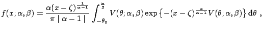
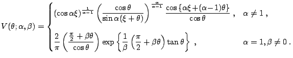
The direct integration method, proposed by Nolan 1997, 1999) consists of a numerical integration of Zolotarev's (1986) formulas for the density or the distribution function. To save space we state only the formulas for the probability density function. Complete formulas can be also found in [12].

Set $\zeta = -\beta\tan\frac{\pi\alpha}{2}$. Then the density $f(x;\alpha,\beta)$ of a standard $\alpha$-stable random variable in representation $S^0$, i.e. $X\sim S^0_{\alpha}(1,\beta,0)$, can be expressed as (note, that Zolotarev 1986, Sect. 2.2) used yet another parametrization):

• when $\alpha\ne 1$ and $x>\zeta$:

  $$f(x;\alpha,\beta) = \frac{\alpha(x-\zeta)^{\frac{1}{\alpha-1}}} {... ...ta)^{\frac{\alpha}{\alpha-1}}V(\theta;\alpha,\beta)\right\} {\text{d}}\theta\;,$$

  
  

• when $\alpha\ne 1$ and $x=\zeta$:

  $$f(x;\alpha,\beta) = \frac{\Gamma\left(1+\frac{1}{\alpha}\right) \cos(\xi)} {\pi(1+\zeta^2)^{\frac{1}{2\alpha}}}\;,$$

  
  

• when $\alpha\ne 1$ and $x<\zeta$:

  $$f(x;\alpha,\beta) = f(-x;\alpha,-\beta)\;,$$

  
  

• when $\alpha=1$:

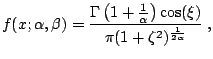  $$f(x;1,\beta)= \begin{cases}\displaystyle \frac{1}{2\mid\beta\mid}... ...ne 0\;, \\ [4mm] \displaystyle \frac{1}{\pi(1+x^2)}\;, & \beta=0\;, \end{cases}$$

  
  

where

$$\xi =\begin{cases}\displaystyle \frac{1}{\alpha} \arctan(-\zeta)\... ...lpha \ne 1\;, \\ [4mm] \displaystyle \frac{\pi}{2}\;, & \alpha=1\;, \end{cases}$$ (1.5)

and

$$V(\theta;\alpha,\beta) = \begin{cases}\displaystyle (\cos\alpha\x... ...+\beta\theta\right)\tan\theta\right\}\;, & \alpha=1, \beta \ne 0\;. \end{cases}$$

XploRe offers the direct integration method through the cdfstab and pdfstab quantlets, see [22] for a thorough exposition of quantlets related to stable distributions. On a PC equipped with a Centrino $1.6\,$GHz processor the calculation of the stable distribution or density function at $1000$ points takes about $1.2$ seconds. As default, the integrals found in the above formulas are numerically integrated using $2000$ subintervals. These computational times can be improved when using a numerically more efficient environment. For example, the program STABLE (downloadable from John Nolan's web page: http://academic2.american.edu/~jpnolan/stable/stable.html) needs about $0.9$ seconds for performing corresponding calculations. It was written in Fortran and calls several external IMSL routines, see [79] for details. Apart from speed, the STABLE program also exhibits higher relative accuracy (for default tolerance settings in both programs): about $10^{-13}$ compared to $10^{-10}$ for values used in typical financial applications (like approximating asset return distributions). Naturally, the accuracy of both programs can be increased at the cost of computational time.

It is interesting to note, that currently no other statistical computing environment offers the computation of stable density and distribution functions in its standard release. Users have to rely on third-party libraries or commercial products. A few are worth mentioning. John Nolan offers the STABLE program in library form through Robust Analysis Inc., see http://www.robustanalysis.com. This library (in C, Visual Basic or Fortran) provides interfaces to Matlab, S-plus (or its GNU version - R) and Mathematica. Diethelm Würtz has developed Rmetrics, an open source collection of software packages for S-plus/R, which may be useful for teaching computational finance, see http://www.itp.phys.ethz.ch/econophysics/R/. Stable PDF and CDF calculations are performed using the direct integration method, with the integrals being computed by R's function integrate. Interestingly, for symmetric stable distributions Rmetrics utilizes McCulloch's (1998) approximation, which was obtained by interpolating between the complements of the Cauchy and Gaussian CDFs in a transformed space. For $\alpha>0.92$ the absolute precision of the stable PDF and CDF approximation is $10^{-4}$. The FFT based approach is utilized in Cognity, a commercial risk management platform that offers derivatives pricing and portfolio optimization based on the assumption of stably distributed returns, see http://www.finanalytica.com.

1.2.3 Simulation of $\alpha$-stable Variables

The complexity of the problem of simulating sequences of $\alpha$-stable random variables stems from the fact that there are no analytic expressions for the inverse $F^{-1}(x)$ nor the cumulative distribution function $F(x)$. All standard approaches like the rejection or the inversion methods would require tedious computations. See Chap. II.2 for a review of non-uniform random number generation techniques.

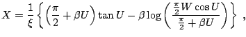
A much more elegant and efficient solution was proposed by [21]. They noticed that a certain integral formula derived by [100] yielded the following algorithm:

• generate a random variable $U$ uniformly distributed on $\left(-\frac{\pi}{2},\frac{\pi}{2}\right)$ and an independent exponential random variable $W$ with mean $1$;

• for $\alpha\ne 1$ compute:

  $$X = (1+\zeta^2)^{\frac{1}{2\alpha}} \frac{\sin\{ \alpha(U+\xi)\}}... ...\left[\frac{\cos\{U - \alpha(U+\xi) \}}{W} \right]^{\frac{1-\alpha}{\alpha}}\;,$$ (1.6)

  
  

• for $\alpha=1$ compute:

  $$X = \frac{1}{\xi}\left\{\left(\frac{\pi}{2}+\beta U \right)\tan U... ...\log\left(\frac{\frac{\pi}{2} W\cos U}{\frac{\pi}{2}+\beta U}\right)\right\}\;,$$ (1.7)

  
  

where $\xi$ is given by (1.5). This algorithm yields a random variable $X\sim S_{\alpha}(1,\beta,0)$, in representation (1.3). For a detailed proof see [98].

Given the formulas for simulation of a standard $\alpha$-stable random variable, we can easily simulate a stable random variable for all admissible values of the parameters $\alpha$, $\sigma$, $\beta$ and $\mu$ using the following property: if $X\sim S_{\alpha}(1,\beta,0)$ then

$$Y=\begin{cases}\sigma X+\mu\;, & \alpha \ne 1\;, \\ [2mm] \displa... ... \sigma X+\frac{2}{\pi}\beta\sigma\log\sigma + \mu\;, & \alpha=1\;, \end{cases}$$

is $S_{\alpha}(\sigma,\beta,\mu)$. It is interesting to note that for $\alpha = 2$ (and $\beta = 0$) the Chambers-Mallows-Stuck method reduces to the well known [14] algorithm for generating Gaussian random variables ([49]).

Many other approaches have been proposed in the literature, including application of [8] and LePage ([60]) series expansions, see [65] and [47], respectively. However, this method is regarded as the fastest and the most accurate. In XploRe the algorithm is implemented in the rndstab quantlet. On a PC equipped with a Centrino $1.6\,$GHz processor one million variables are generated in about $3$ seconds, compared to about $0.4$ seconds for one million standard normal random variables obtained via the Box-Muller algorithm (normal2). Because of its unquestioned superiority and relative simplicity, the Chambers-Mallows-Stuck method is implemented in some statistical computing environments (e.g. the rstable function in S-plus/R) even if no other routines related to stable distributions are provided.

1.2.4 Estimation of Parameters

The estimation of stable law parameters is in general severely hampered by the lack of known closed-form density functions for all but a few members of the stable family. Numerical approximation or direct numerical integration are nontrivial and burdensome from a computational point of view. As a consequence, the maximum likelihood (ML) estimation algorithm based on such approximations is difficult to implement and time consuming for samples encountered in modern finance. However, there are also other numerical methods that have been found useful in practice and are discussed in this section.

All presented methods work quite well assuming that the sample under consideration is indeed $\alpha$-stable. Since there are no formal tests for assessing the $\alpha$-stability of a data set we suggest to first apply the ''visual inspection'' and tail exponent estimators to see whether the empirical densities resemble those of $\alpha$-stable laws ([12,99]).

Given a sample $x_1, \ldots, x_n$ of independent and identically distributed (i.i.d.) $S_{\alpha}(\sigma,\beta,\mu)$ observations, in what follows, we provide estimates $\hat{\alpha}$, $\hat{\sigma}$, $\hat{\beta}$ and $\hat{\mu}$ of all four stable law parameters. We start the discussion with the simplest, fastest and $\ldots$ least accurate quantile methods, then develop the slower, yet much more accurate sample characteristic function methods and, finally, conclude with the slowest but most accurate maximum likelihood approach.

1.2.4.1 Sample Quantile Methods

[37] provided very simple estimates for parameters of symmetric ( $\beta=0, \mu=0$) stable laws with $\alpha>1$. They proposed to estimate $\sigma$ by:

$$\hat{\sigma} = \frac{\hat{x}_{0.72} - \hat{x}_{0.28}}{1.654}\;,$$ (1.8)

where $x_f$ denotes the $f$-th population quantile, so that $S_{\alpha}(\sigma,\beta,\mu)(x_f) = f$. As [70] noticed, Fama and Roll based their estimator of $\sigma$ on the fortuitous observation that $(x_{0.72}-x_{0.28})/\sigma$ lies within $0.4\,{\%}$ of $1.654$ for all $1<\alpha\le 2$, when $\beta = 0$. This enabled them to estimate $\sigma$ by (1.8) with less than $0.4\,{\%}$ asymptotic bias without first knowing $\alpha$. However, when $\beta\ne 0$, the search for an invariant range such as the one they found becomes futile.

The characteristic exponent $\alpha$, on the other hand, can be estimated from the tail behavior of the distribution. Fama and Roll suggested to take  $\hat{\alpha}$ satisfying:

$$S_{\hat{\alpha}}\left(\frac{\hat{x}_f - \hat{x}_{1-f}}{2\hat{\sigma}}\right) = f\;.$$ (1.9)

They found that $f=0.95$, $0.96$, $0.97$ worked best for estimating $\alpha$. This method unnecessarily compounds the small asymptotic bias in the estimator of $\sigma$ into the estimator of $\alpha$.

For $1<\alpha\le 2$, the stable distribution has finite mean. Hence, the sample mean is a consistent estimate of the location parameter $\mu$. However, a more robust estimate is the $p\%$ truncated sample mean - the arithmetic mean of the middle $p$ percent of the ranked observations. The $50\,{\%}$ truncated mean is often suggested in the literature when the range of $\alpha$ is unknown.

Fama and Roll's (1971) method is simple but suffers from a small asymptotic bias in $\hat{\alpha}$ and $\hat{\sigma}$ and restrictions on $\alpha$ and $\beta$. [70] generalized and improved the quantile method. He analyzed stable law quantiles and provided consistent estimators of all four stable parameters, with the restriction $\alpha\ge 0.6$, while retaining the computational simplicity of Fama and Roll's method. After McCulloch define:

$$v_{\alpha}=\frac{x_{0.95}-x_{0.05}}{x_{0.75}-x_{0.25}} \quad v_{\beta}=\frac{x_{0.95}+x_{0.05}-2x_{0.50}}{x_{0.95}-x_{0.05}}\;.$$ (1.10)

Statistics $v_{\alpha}$ and $v_{\beta}$ are functions of $\alpha$ and $\beta$ only, i.e. they are independent of both $\sigma$ and $\mu$. This relationship may be inverted and the parameters $\alpha$ and $\beta$ may be viewed as functions of $v_{\alpha}$ and $v_{\beta}$. Substituting $v_{\alpha}$ and $v_{\beta}$ by their sample values and applying linear interpolation between values found in tables given in [70] yields estimators $\hat{\alpha}$ and  $\hat{\beta}$.

Scale and location parameters, $\sigma$ and $\mu$, can be estimated in a similar way. However, due to the discontinuity of the characteristic function for $\alpha=1$ and $\beta\ne 0$ in representation (1.3), this procedure is more complicated. We refer the interested reader to the original work of [70]. This estimation technique is implemented in XploRe in the stabcull quantlet.

1.2.4.2 Sample Characteristic Function Methods

Given an i.i.d. random sample $x_1, \ldots, x_n$ of size $n$, define the sample characteristic function by:

$$\hat{\phi}(t) = \frac{1}{n} \sum_{j=1}^{n} \exp(itx_j)\;.$$

Since $\vert\hat{\phi}(t)\vert$ is bounded by unity all moments of $\hat{\phi}(t)$ are finite and, for any fixed $t$, it is the sample average of i.i.d. random variables $\exp(itx_j)$. Hence, by the law of large numbers, $\hat{\phi}(t)$ is a consistent estimator of the characteristic function $\phi(t)$.

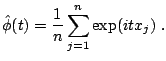[85] proposed a simple estimation method, called the method of moments, based on transformations of the characteristic function. From (1.3) we have for all $\alpha$:

$$\vert\phi(t)\vert=\exp(-\sigma^{\alpha} \vert t\vert^{\alpha})\;.$$ (1.11)

Hence, $-\log\vert\phi(t)\vert=\sigma^{\alpha} \vert t\vert^{\alpha}$. Now, assuming $\alpha\ne 1$, choose two nonzero values of $t$, say $t_1 \ne t_2$. Then for $k=1,2$ we have:

$$-\log\vert\phi(t_k)\vert=\sigma^{\alpha} \vert t_k\vert^{\alpha}\;.$$ (1.12)

Solving these two equations for $\alpha$ and $\sigma$, and substituting $\hat{\phi}(t)$ for $\phi(t)$ yields:

$$\hat{\alpha}=\frac{\log \frac{\log\vert\hat{\phi}(t_1)\vert}{\log\vert\hat{\phi}(t_2)\vert}} {\log\left\vert\frac{t_1}{t_2}\right\vert}\;,$$ (1.13)

and

$$\log\hat{\sigma}=\frac{\log\vert t_1\vert\log(-\log\vert\hat{\phi... ...g(-\log\vert\hat{\phi}(t_1)\vert)}{\log\left\vert\frac{t_1}{t_2}\right\vert}\;.$$ (1.14)

In order to estimate $\beta$ and $\mu$ we have to choose two nonzero values of $t$, say $t_3 \ne t_4$, and apply a similar trick to $\Im\{\log \phi(t)\}$. The estimators are consistent since they are based upon estimators of $\phi(t)$, $\Im\{\phi(t)\}$ and $\Re\{\phi(t)\}$, which are known to be consistent. However, convergence to the population values depends on the choice of $t_1,\ldots,t_4$. The optimal selection of these values is problematic and still is an open question. The XploRe implementation of the method of moments (the stabmom quantlet) uses $t_1=0.2$, $t_2=0.8$, $t_3=0.1$, and $t_4=0.4$ as proposed by [56] in his simulation study.

In the same paper Koutrouvelis presented a much more accurate regression-type method which starts with an initial estimate of the parameters and proceeds iteratively until some prespecified convergence criterion is satisfied. Each iteration consists of two weighted regression runs. The number of points to be used in these regressions depends on the sample size and starting values of $\alpha$. Typically no more than two or three iterations are needed. The speed of the convergence, however, depends on the initial estimates and the convergence criterion.

The regression method is based on the following observations concerning the characteristic function $\phi(t)$. First, from (1.3) we can easily derive:

$$\log\left(-\log\vert\phi(t)\vert^{2}\right)=\log\left(2\sigma^{\alpha}\right)+\alpha\log\vert t\vert\;.$$ (1.15)

The real and imaginary parts of $\phi(t)$ are for $\alpha\ne 1$ given by:

$$\Re\{\phi(t)\}=\exp(-\vert\sigma t\vert^{\alpha}) \cos\left[\mu t+\vert\sigma t\vert^{\alpha} \beta \text{sign}(t)\tan\frac{\pi\alpha}{2}\right]\;,$$

and

$$\Im\{\phi(t)\}=\exp(-\vert\sigma t\vert^{\alpha}) \sin\left[\mu t+\vert\sigma t\vert^{\alpha} \beta \text{sign}(t)\tan\frac{\pi\alpha}{2}\right]\;.$$

The last two equations lead, apart from considerations of principal values, to:

$$\arctan\left(\frac{\Im\{\phi(t)\}}{\Re\{\phi(t)\}}\right) =\mu t+\beta\sigma^{\alpha} \tan\frac{\pi\alpha}{2} (t) \vert t\vert^{\alpha}\;.$$ (1.16)

Equation (1.15) depends only on $\alpha$ and $\sigma$ and suggests that we estimate these parameters by regressing $y_k=\log(-\log\vert\hat{\phi}(t_k)\vert^{2})$ on $w_k=\log\vert t_k\vert$ in the model:

$$y_k=m+\alpha w_k + \epsilon_k\;,$$ (1.17)

where $\{t_k\}$ is an appropriate set of real numbers, $m=\log(2\sigma^{\alpha})$, and $\epsilon_k$ denotes an error term. [56] proposed to use $t_{k}=\frac{\pi k}{25}, k=1,2,\ldots,K$; with $K$ ranging between $9$ and $134$ for different values of $\alpha$ and sample sizes.

Once $\hat{\alpha}$ and $\hat{\sigma}$ have been obtained and $\alpha$ and $\sigma$ have been fixed at these values, estimates of $\beta$ and $\mu$ can be obtained using (1.16). Next, the regressions are repeated with $\hat{\alpha}$, $\hat{\sigma}$, $\hat{\beta}$ and $\hat{\mu}$ as the initial parameters. The iterations continue until a prespecified convergence criterion is satisfied. Koutrouvelis proposed to use the Fama-Roll estimator (1.8) and the $25\,{\%}$ truncated mean for initial estimates of $\sigma$ and $\mu$, respectively.

[54] eliminated this iteration procedure and simplified the regression method. For initial estimation they applied McCulloch's method, worked with the continuous representation (1.4) of the characteristic function instead of the classical one (1.3) and used a fixed set of only 10 equally spaced frequency points $t_k$. In terms of computational speed their method compares favorably to the original method of Koutrouvelis, see Table 1.1. It has a significantly better performance near $\alpha=1$ and $\beta\ne 0$ due to the elimination of discontinuity of the characteristic function. However, it returns slightly worse results for other values of $\alpha$. In XploRe both regression algorithms are implemented in the stabreg quantlet. An optional parameter lets the user choose between the original Koutrouvelis code and the Kogon-Williams modification.

Table 1.1: Comparison of McCulloch's quantile technique, the method of moments, the regression approach of Koutrouvelis and the method of Kogon and Williams for 100 simulated samples of two thousand $S_{1.7}$ (0.005, 0.1, 0.001) random numbers each. Parameter estimates are mean values over 100 samples. Values of the Mean Absolute Percentage Error (MAPE $_{\theta} = \frac{1}{n} \sum_{i=1}^n \vert \hat{\theta} - \theta\vert / \theta$) are given in parentheses. In the last column average computational times for one sample of 2000 random variables are provided (on a PC equipped with a Centrino 1.6 GHz processor and running XploRe 4.6) (Q: CSAfin03)

Method	$\hat{\alpha}$	$\hat{\sigma}$	$\hat{\beta}$	$\hat{\mu}$	CPU time
McCulloch	$1.7005$	$0.0050$	$0.1045$	$0.0010$	$0.025\,$s
	( $2.60\,{\%}$)	( $2.16\,{\%}$)	( $110.72\,{\%}$)	( $22.01\,{\%}$)
Moments	$1.9895$	$0.0104$	$0.0712$	$0.0010$	$0.015\,$s
	( $17.03\,{\%}$)	( $107.64\,{\%}$)	( $969.57\,{\%}$)	( $33.56\,{\%}$)
Koutrouvelis	$1.6988$	$0.0050$	$0.0989$	$0.0010$	$0.300\,$s
	( $1.66\,{\%}$)	( $1.69\,{\%}$)	( $108.21\,{\%}$)	( $21.01\,{\%}$)
Kogon-Williams	$1.6994$	$0.0050$	$0.0957$	$0.0010$	$0.085\,$s
	( $1.95\,{\%}$)	( $1.77\,{\%}$)	( $110.59\,{\%}$)	( $21.14\,{\%}$)

A typical performance of the described estimators is summarized in Table 1.1, see also Fig. 1.5. McCulloch's quantile technique, the method of moments, the regression approach of Koutrouvelis and the method of Kogon and Williams were applied to 100 simulated samples of two thousand $S_{1.7}(0.005, 0.1, 0.001)$ random numbers each. The method of moments yielded the worst estimates, clearly outside any admissible error range. McCulloch's method came in next with acceptable results and computational time significantly lower than the regression approaches. On the other hand, both the Koutrouvelis and the Kogon-Williams implementations yielded good estimators with the latter performing considerably faster, but slightly less accurate. We have to say, though, that all methods had problems with estimating $\beta$. Like it or not, our search for the optimal estimation technique is not over yet. We have no other choice but turn to the last resort - the maximum likelihood method.

Figure 1.5: Regression fit (dashed), using Koutrouvelis' regression method, to 2000 simulated $S_{1.7}(0.005, 0.1, 0.001)$ random variables (circles). For comparison, the CDF of the original distribution is also plotted (solid). The right panel is a magnification of the left tail fit on a double logarithmic scale (Q: CSAfin04)

1.2.4.3 Maximum Likelihood Method

The maximum likelihood (ML) estimation scheme for $\alpha$-stable distributions does not differ from that for other laws, at least as far as the theory is concerned. For a vector of observations $x=(x_1,\ldots,x_n)$, the ML estimate of the parameter vector $\theta=(\alpha, \sigma, \beta, \mu)$ is obtained by maximizing the log-likelihood function:

$$L_{\theta}(x) = \sum_{i=1}^n \log \tilde{f}(x_i; \theta)\,,$$ (1.18)

where $\tilde{f}(\cdot; \theta)$ is the stable density function. The tilde denotes the fact that, in general, we do not know the explicit form of the stable PDF and have to approximate it numerically. The ML methods proposed in the literature differ in the choice of the approximating algorithm. However, all of them have an appealing common feature - under certain regularity conditions the maximum likelihood estimator is asymptotically normal with the variance specified by the Fischer information matrix ([30]). The latter can be approximated either by using the Hessian matrix arising in maximization or, as in [81], by numerical integration.

Because of computational complexity there are only a few documented attempts of estimating stable law parameters via maximum likelihood. [29] developed an approximate ML method, which was based on grouping the data set into bins and using a combination of means to compute the density (FFT for the central values of $x$ and series expansions for the tails) to compute an approximate log-likelihood function. This function was then numerically maximized.

Applying Zolotarev's (1964) integral formulas, [17] formulated another approximate ML method, however, only for symmetric stable random variables. To avoid the discontinuity and nondifferentiability of the symmetric stable density function at $\alpha=1$, the tail index $\alpha$ was restricted to be greater than one.

Much better, in terms of accuracy and computational time, are more recent maximum likelihood estimation techniques. [76] utilized the FFT approach for approximating the stable density function, whereas [81] used the direct integration method. Both approaches are comparable in terms of efficiency. The differences in performance are the result of different approximation algorithms, see Sect. 1.2.2.

As [83] observes, the ML estimates are almost always the most accurate, closely followed by the regression-type estimates, McCulloch's quantile method, and finally the method of moments. However, as we have already said in the introduction to this section, maximum likelihood estimation techniques are certainly the slowest of all the discussed methods. For example, ML estimation for a sample of $2000$ observations using a gradient search routine which utilizes the direct integration method needs $221$ seconds or about $3.7$ minutes! The calculations were performed on a PC equipped with a Centrino ${1.6}\,$GHz processor and running STABLE ver. $3.13$ (see also Sect. 1.2.2 where the program was briefly described). For comparison, the STABLE implementation of the Kogon-Williams algorithm performs the same calculations in only $0.02$ seconds (the XploRe quantlet stabreg needs roughly four times more time, see Table 1.1). Clearly, the higher accuracy does not justify the application of ML estimation in many real life problems, especially when calculations are to be performed on-line. For this reason the program STABLE also offers an alternative - a fast quasi ML technique. It quickly approximates stable densities using a $3$-dimensional spline interpolation based on pre-computed values of the standardized stable density on a grid of $(x,\alpha,\beta)$ values. At the cost of a large array of coefficients, the interpolation is highly accurate over most values of the parameter space and relatively fast - $0.26$ seconds for a sample of $2000$ observations.

Table 1.2: $\alpha$-stable and Gaussian fits to $2000$ returns of the Dow Jones Industrial Average (DJIA) index from the period January 2, 1985 - November 30, 1992. Values of the Anderson-Darling and Kolmogorov goodness-of-fit statistics suggest a much better fit of the $1.66$-stable law. Empirical and model based ($\alpha$-stable and Gaussian) VaR numbers at the 95 % and 99 % confidence levels are also given. The values in parentheses are the relative differences between model and empirical VaR estimates (Q: CSAfin05)

Parameters	$\alpha$	$\sigma$	$\beta$	$\mu$
$\alpha$-stable fit	$1.6596$	$0.0053$	$0.0823$	$0.0009$
Gaussian fit		$0.0115$		$0.0006$
Test values	Anderson-Darling		Kolmogorov
$\alpha$-stable fit	$1.0044$		$0.8641$
Gaussian fit	$+$INF		$4.5121$
VaR estimates ( $\times 10^{-2}$)	$95\,{\%}$		$99\,{\%}$
Empirical	$1.5242$		$2.8922$
$\alpha$-stable fit	$1.3296$	( $12.77\,{\%}$)	$2.7480$	( $4.98\,{\%}$)
Gaussian fit	$1.8350$	( $20.39\,{\%}$)	$2.6191$	( $9.44\,{\%}$)

Figure 1.6: $1.66$-stable (solid grey line) and Gaussian (dashed line) fits to the DJIA returns (circles) empirical cumulative distribution function from the period January 2, 1985 - November 30, 1992. For better exposition of the fit in the central part of the distribution ten largest and ten smallest returns are not illustrated in the left panel. The right panel is a magnification of the left tail fit on a double logarithmic scale. Vertical lines represent the $1.66$-stable (solid grey line), Gaussian (dashed line) and empirical (solid line) VaR estimates at the 95 % (filled circles, triangles and squares) and 99 % (hollow circles, triangles and squares) confidence levels (Q: CSAfin05)

1.2.5 Are Asset Returns $\alpha$-stable?

In this paragraph we want to apply the discussed techniques to financial data. Due to limited space we have chosen only one estimation method - the regression approach of [56], as it offers high accuracy at moderate computational time. We start the empirical analysis with the most prominent example - the Dow Jones Industrial Average (DJIA) index. The data set covers the period January 2, 1985 - November 30, 1992 and comprises $2000$ returns. Recall, that this period includes the largest crash in Wall Street history - the Black Monday of October 19, 1987. Clearly the $1.66$-stable law offers a much better fit to the DJIA returns than the Gaussian distribution, see Table 1.2. Its superiority, especially in the tails of the distribution, is even better visible in Fig.  1.6. In this figure we also plotted vertical lines representing the $1.66$-stable, Gaussian and empirical daily VaR estimates at the $c = 95\,{\%}$ and $99\,{\%}$ confidence levels. These estimates correspond to a one day VaR of a virtual portfolio consiting of one long position in the DJIA index. The stable VaR estimates are almost twice closer to the empirical estimates than the Gaussian ones, see Table 1.2.

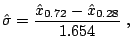
Recall that calculating the VaR number reduces to finding the $(1-c)$ quantile of a given distribution or equivalently to evaluating the inverse $F^{-1}$ of the distribution function at $(1-c)$. Unfortunately no simple algorithms for inverting the stable CDF are known. The qfstab quantlet of XploRe utilizes a simple binary search routine for large $\alpha$'s and values near the mode of the distribution. In the extreme tails the approximate range of the quantile values is first estimated via the power law formula (1.1), then a binary search is conducted.

To make our statistical analysis more sound, we also compare both fits through Anderson-Darling and Kolmogorov test statistics ([24]). The former may be treated as a weighted Kolmogorov statistics which puts more weight to the differences in the tails of the distributions. Although no asymptotic results are known for the stable laws, approximate critical values for these goodness-of-fit tests can be obtained via the bootstrap technique ([12,94]). In this chapter, though, we will not perform hypothesis testing and just compare the test values. Naturally, the lower the values the better the fit. The stable law seems to be tailor-cut for the DJIA index returns. But does it fit other asset returns as well?

The second analyzed data set comprises $2000$ returns of the Deutsche Aktienindex (DAX) index from the period January 2, 1995 - December 5, 2002. Also in this case the $\alpha$-stable law offers a much better fit than the Gaussian, see Table 1.3. However, the test statistics suggest that the fit is not as good as for the DJIA returns (observe that both data sets are of the same size and the test values in both cases can be compared). This can be also seen in Fig. 1.7. The left tail seems to drop off at some point and the very tail is largely overestimated by the stable distribution. At the same time it is better approximated by the Gaussian law. This results in a surprisingly good fit of the daily $95\,{\%}$ VaR by the Gaussian distribtion, see Table 1.3, and an overestimation of the daily VaR estimate at the $c = 99\,{\%}$ confidence level by the $1.7$-stable distribtion. In fact, the latter is a rather typical situation. For a risk manager who likes to play safe this may not be a bad idea, as the stable law overestimates the risks and thus provides an upper limit of losses.

Table 1.3: $\alpha$-stable and Gaussian fits to 2000 returns of the Deutsche Aktienindex (DAX) index from the period January 2, 1995 - December 5, 2002. Empirical and model based ($\alpha$-stable and Gaussian) VaR numbers at the 95% and 99% confidence levels are also given (Q: CSAfin06)

Parameters	$\alpha$	$\sigma$	$\beta$	$\mu$
$\alpha$-stable fit	$1.7003$	$0.0088$	$-0.3179$	$-0.0002$
Gaussian fit		$0.0157$		$0.0004$
Test values	Anderson-Darling		Kolmogorov
$\alpha$-stable fit	$1.9149$		$1.1798$
Gaussian fit	$16.4119$		$2.8197$
VaR estimates ( $\times 10^{-2}$)	$95\,{\%}$		$99\,{\%}$
Empirical	$2.5731$		$4.5963$
$\alpha$-stable fit	$2.4296$	( $5.58\,{\%}$)	$5.0982$	( $10.92\,{\%}$)
Gaussian fit	$2.5533$	( $0.77\,{\%}$)	$3.6260$	( $21.11\,{\%}$)

Figure 1.7: $1.7$-stable (solid grey line) and Gaussian (dashed line) fits to the DAX returns (black circles) empirical cumulative distribution function from the period January 2, 1995 - December 5, 2002. For better exposition of the fit in the central part of the distribution ten largest and ten smallest returns are not illustrated in the left panel. The right panel is a magnification of the left tail fit on a double logarithmic scale. Vertical lines represent the $1.7$-stable (solid grey line), Gaussian (dashed line) and empirical (solid black line) VaR estimates at the 95 % (filled circles, triangles and squares) and 99 % (hollow circles, triangles and squares) confidence levels. This time the stable law overestimates the tails of the empirical distribution (Q: CSAfin06)

This example clearly shows that the $\alpha$-stable distribution is not a panacea. Although it gives a very good fit to a number of empirical data sets, there surely are distributions that recover the characteristics of other data sets better. We devote the rest of this chapter to such alternative heavy tailed distributions. We start with a modification of the stable law and in Sect. 1.3 concentrate on the class of generalized hyperbolic distributions.

1.2.6 Truncated Stable Distributions

Mandelbrot's (1963) pioneering work on applying $\alpha$-stable distributions to asset returns gained support in the first few years after its publication ([36,82,95]). Subsequent works, however, have questioned the stable distribution hypothesis ([1,11]). By the definition of the stability property, the sum of i.i.d. stable random variables is also stable. Thus, if short term asset returns are distributed according to a stable law, longer term returns should retain the same functional form. However, from the empirical data it is evident that as the time interval between price observations grows longer, the distribution of returns deviates from the short term heavy tailed distribution, and converges to the Gaussian law. This indicates that the returns probably are not $\alpha$-stable (but it could mean as well that the returns are just not independent). Over the next few years, the stable distribution temporarily lost favor and alternative processes were suggested as mechanisms generating stock returns.

In mid 1990s the stable distribution hypothesis has made a dramatic comeback. Several authors have found a very good agreement of high-frequency returns with a stable distribution up to six standard deviations away from the mean ([23,67]). For more extreme observations, however, the distribution they have found falls off approximately exponentially. To cope with such observations the truncated Lévy distributions (TLD) were introduced by [66]. The original definition postulated a sharp truncation of the $\alpha$-stable probability density function at some arbitrary point. However, later an exponential smoothing was proposed by [55].

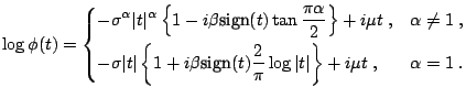
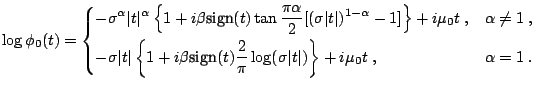
For $\alpha\ne 1$ the characteristic function of a symmetric TLD random variable is given by:

$$\log\phi(t) = -\frac{\sigma^{\alpha}}{\cos\frac{\pi\alpha}{2}} \l... ...pha \arctan \frac{\vert t\vert}{\lambda} \right\} - \lambda^{\alpha} \right]\;,$$

where $\alpha$ is the tail exponent, $\sigma$ is the scale parameter and $\lambda$ is the truncation coefficient. Clearly the TLD reduces to the symmetric $\alpha$-stable distribution ( $\beta =\mu =0$) when $\lambda=0$. The TLD distribution exhibits the following behavior: for small and intermediate returns it behaves like a stable distribution, but for extreme returns the truncation causes the distribution to converge to a Gaussian distribution. Thus the observation that the asset returns distribution is a TLD explains both the short-term $\alpha$-stable behavior and the long run convergence to the normal distribution.

Despite these interesting features the truncated Lévy distributions have not been applied extensively to date. The most probable reason for this being the complicated definition of the TLD law. Like for $\alpha$-stable distributions, only the characteristic function is known. No closed form formulas exist for the density or the distribution function. Since no integral formulas, like Zolotarev's (1986) for the $\alpha$-stable laws, have been discovered as yet, statistical inference is, in general, limited to maximum likelihood utilizing the FFT technique for approximating the PDF. Moreover, compared to the stable distribution, the TLD introduces one more parameter (asymmetric TLD laws have also been considered in the literature, see e.g. [15] and [55]) making the estimation procedure even more complicated. Other parameter fitting techniques proposed so far comprise a combination of ad hoc approaches and moment matching ([15,69]). Better techniques have to be discovered before TLDs become a common tool in finance.