Next: 3.7 Sampler Performance and
Up: 3. Markov Chain Monte
Previous: 3.5 MCMC Sampling with
3.6 Estimation of Density Ordinates
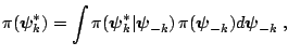
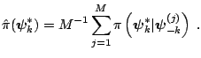
We mention that if the full conditional densities are available,
whether in the context of the multiple-block M-H algorithm or that of
the Gibbs sampler, then the MCMC output can be used to estimate
posterior marginal density functions ([58,23]). We
exploit the fact that the marginal density of
 at
the point
at
the point
 is
is
where as before
 . Provided the normalizing constant of
 is known,
an estimate of the marginal density is available as an average of the
full conditional density over the simulated values
of
is known,
an estimate of the marginal density is available as an average of the
full conditional density over the simulated values
of
 :
:
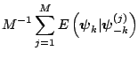
Under the assumptions of Proposition 1,
 as as |
|
[23] refer to this approach as
Rao-Blackwellization because of the connections with the
Rao-Blackwell theorem in classical statistics. That connection is more
clearly seen in the context of estimating (say) the mean of
,
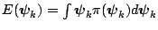 . By the law of the iterated
expectation,
. By the law of the iterated
expectation,
and therefore the estimates
and
both converge to
 as
as
 . Under
  sampling, and under Markov sampling provided some
conditions are satisfied - see [35], [6] and
[50], it can be shown that the variance of the latter
estimate is smaller than that of the former. Thus, it can help to
average the conditional mean
sampling, and under Markov sampling provided some
conditions are satisfied - see [35], [6] and
[50], it can be shown that the variance of the latter
estimate is smaller than that of the former. Thus, it can help to
average the conditional mean
 if that were available,
rather than average the draws directly. [23] appeal to
this analogy to argue that the Rao-Blackwellized estimate of the
density is preferable to that based on the method of kernel smoothing.
[11] extends the Rao-Blackwellization approach to estimate
reduced conditional ordinates defined as the density of
conditioned on one or more of the remaining
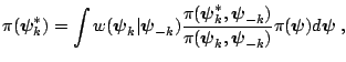
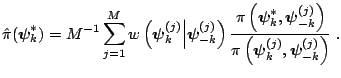
blocks. Finally, [9] provides an importance weighted
estimate of the marginal density for cases where the conditional
posterior density does not have a known normalizing constant. Chen's
estimator is based on the identity
if that were available,
rather than average the draws directly. [23] appeal to
this analogy to argue that the Rao-Blackwellized estimate of the
density is preferable to that based on the method of kernel smoothing.
[11] extends the Rao-Blackwellization approach to estimate
reduced conditional ordinates defined as the density of
conditioned on one or more of the remaining
blocks. Finally, [9] provides an importance weighted
estimate of the marginal density for cases where the conditional
posterior density does not have a known normalizing constant. Chen's
estimator is based on the identity
where
 is a completely known
conditional density whose support is equal to the support of the full
conditional density
is a completely known
conditional density whose support is equal to the support of the full
conditional density
 . In
this form, the normalizing constant of the full conditional density is
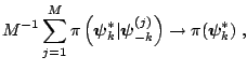
not required and given a sample of draws
. In
this form, the normalizing constant of the full conditional density is
not required and given a sample of draws
 from
from
 , a Monte Carlo estimate of the marginal density is
given by
, a Monte Carlo estimate of the marginal density is
given by
[9] discusses the choice of the conditional
density  . Since it depends on
, the choice of
will vary from one sampled draw to the next.
. Since it depends on
, the choice of
will vary from one sampled draw to the next.
Next: 3.7 Sampler Performance and
Up: 3. Markov Chain Monte
Previous: 3.5 MCMC Sampling with