Subsections

• 4.5.1 Storage Schemes for Sparse Matrices
• 4.5.2 Methods for Sparse Matrices

4.5 Sparse Matrices

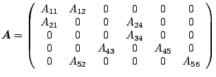
Numerical problems arising in some applications, such as seemingly unrelated regressions, spatial statistics, or support vector machines (Chap. III.15), are sparse: they often involve large matrices, which have only a small number of nonzero elements. (It is difficult to specify what exactly ''small number'' is.) From the practical point of view, a matrix is sparse if it has so many zero elements that it is worth to inspect their structure and use appropriate methods to save storage and the number of operations. Some sparse matrices show a regular pattern of nonzero elements (e.g., band matrices), while some exhibit a rather irregular pattern. In both cases, solving the respective problem efficiently means to store and operate on only nonzero elements and to keep the ''fill,'' the number of newly generated nonzero elements, as small as possible.

In this section, we first discuss some of storage schemes for sparse matrices, which could indicate what types of problems can be effectively treated as sparse ones (Sect. 4.5.1). Later, we give examples of classical algorithms adopted for sparse matrices (Sect. 4.5.2). Monographs introducing a range of methods for sparse matrices include [12,27] and [54].

4.5.1 Storage Schemes for Sparse Matrices

To save storage, only nonzero elements of a sparse vector or matrix should be stored. There are various storage schemes, which require approximately from two to five times the number of nonzero elements to store a vector or a matrix. Unfortunately, there is no standard scheme. We discuss here the widely used and sufficiently general compressed (row) storage for vectors and for general and banded matrices.

The compressed form of a vector $\boldsymbol {x}$ consists of a triplet $(\boldsymbol{c},\boldsymbol{i},n_0)$, where $\boldsymbol{c}$ is a vector containing nonzero elements of $\boldsymbol {x}$, $\boldsymbol{i}$ is an integer vector containing the indices of elements stored in $\boldsymbol{c}$ and $n_0$ specifies the number of nonzero elements. The stored elements are related to the original vector by formula $x_{\{i_j\}} = c_j$ for $j = 1,\ldots,n_0$. To give an example, the vector $\boldsymbol{x} = (0,0,3,0,-8,1.5,0,0,0,16,0)$ could be stored as

$$\boldsymbol{c} = (3,{1.5},-8,16)\;, \quad \boldsymbol{i} = (3,6,5,10)\;, \quad n_0 = 4\;.$$

Obviously, there is no need to store the elements in the original order. Therefore, adding new nonzero elements is easy. Operations involving more sparse vectors are simpler if we can directly access elements of one vector, that is, if one of the vectors is ''uncompressed.'' For example, computing the inner product $a = \boldsymbol{x}^{\top} \boldsymbol{y}$ of a sparse vector  $\boldsymbol {x}$ stored in the compressed form with a sparse uncompressed vector  $\boldsymbol {y}$ follows the algorithm

$$a = 0\;; \quad j = 1\;,\ldots,n_0\;: \quad a = a + y_{\{i_j\}} \cdot c_j\;.$$

The compressed row storage for matrices is a generalization of the vector concept. We store the nonzero elements of  $\boldsymbol{A}$ as a set of sparse row (or column) vectors in the compressed form. The main difference is that, instead of a single number $n_0$, we need to store a whole vector $\boldsymbol{n}_{0}$ specifying the positions of the first row elements of $\boldsymbol{A}$ in  $\boldsymbol{c}$. For example, the matrix

$$\boldsymbol{A} = \left( \begin{array}{cccccc} A_{11} & A_{12} & 0... ... A_{43} & 0 & A_{45} & 0 \\ 0 & A_{52} & 0 & 0 & 0 & A_{56} \end{array} \right)$$

would be represented rowwise as

$$\boldsymbol{c} = \left(A_{11}, A_{12} \vert A_{21}, A_{24} \vert A_{34} \vert A_{43}, A_{45} \vert A_{52}, A_{56}\right)\;,$$

$$\boldsymbol{i} = (1,2 \vert 1,4 \vert 4 \vert 3,5 \vert 2,6)\;,$$

$$\boldsymbol{n}_{0} = (1,3,5,6,8,10)\;.$$

(The sign ''$\vert$'' just emphasizes the end of a row and has no consequence for the storage itself.) As in the case of vectors, the elements in each row do not have to be ordered. Consequently, there is no direct access to a particular element $A_{ij}$ stored in $\boldsymbol{c}$. Nevertheless, retrieving a row is easy: it suffices to examine the part of $\boldsymbol{i}$ corresponding to the $i$th row, which is given by $\boldsymbol{n}_{0}$. On the contrary, retrieving a column involves a search through the whole storage scheme. Therefore, if a fast access to columns is necessary, it is preferable to simultaneously store $\boldsymbol{A}$ rowwise and columnwise.

A special type of sparse matrices are matrices with a banded structure.

Definition 2   The row bandwidth of a matrix $\boldsymbol{A}\in {\mathbb{R}}^{m\times n}$ is defined as

$$w(\boldsymbol{A}) = \max_{1\le i \le m} \left(l_i(\boldsymbol{A}) - f_i(\boldsymbol{A}) + 1\right)\;,$$

where $f_i(\boldsymbol{A}) = \min\{j\vert\boldsymbol{A}_{ij}\neq 0\}$ and $l_i(\boldsymbol{A}) = \max\{j\vert\boldsymbol{A}_{ij}\neq 0\}$ are column indices of the first and last nonzero elements in the $i$th row of $\boldsymbol{A}$.

A banded matrix $\boldsymbol{A}$ is considered to be sparse if $w(\boldsymbol{A})\ll n$. Contrary to the general case, vector $\boldsymbol{c}$ of a banded matrix typically contains for each row all elements between the first and last nonzero ones. Thus, the storage scheme does not have to include in $\boldsymbol{i}$ all column indices, only one index for the first nonzero element in a row. On the other hand, zeros within the band have to be stored as well. For example, the matrix

$$\boldsymbol{A} = \left( \begin{array}{cccccc} A_{11} & A_{12} & 0... ... 0 \\ 0 & 0 & 0 & A_{34} & 0 \\ 0 & 0 & A_{43} & 0 & A_{45} \end{array} \right)$$

would be represented as

$$\begin{array}{lcl} \displaystyle\boldsymbol{c}&\,=\,&\display... ...\boldsymbol{n}_0&\,=\,&\displaystyle(1,3,6,7,10)\;. \end{array}$$

An interesting observation is that the row bandwidth $w(\boldsymbol{A})$ can be influenced by column permutations. The fill-minimizing column orderings are discussed by [7] and [19], for instance.

Details on some other storage schemes can be found in [12] and [52].

4.5.2 Methods for Sparse Matrices

Methods for sparse matrices are still subject to intensive research. Moreover, the choice of a suitable method for a given problem (and even the choice of an algorithm for elementary operations such as matrix-vector multiplication) depends on many factors, including dimension, matrix type storage scheme, and computational environment (e.g., storage in virtual memory vs. auxiliary storage; vector vs. parallel computing, etc.). Therefore, we provide only a general overview and references to most general results. More details can be found in [7,11,12,27] and [54].

First, many discussed algorithms can be relatively easily adopted for banded matrices. For example, having a row-based storage scheme, one just needs to modify the summation limits in the row version of Cholesky decomposition. Moreover, the positions of nonzero elements can be determined in advance ([49]).

Second, the algorithms for general sparse matrices are more complicated. A graph representation may be used to capture the nonzero pattern of a matrix as well as to predict the pattern of the result (e.g., the nonzero pattern of $\boldsymbol{A}^{\top} \boldsymbol{A}$, the Cholesky factor $\boldsymbol{U}$, etc.). To give an overview, methods adopted for sparse matrices include, but are not limited to, usually used decompositions (e.g., Cholesky, [49]; LU and LDU, [48]; QR, [18], and [32]), solving systems of equations by direct ([26,61]) and iterative methods ([43,68]) and searching eigenvalues ([4,25]).