In this section ![]() is represented by a cloud
of
is represented by a cloud
of ![]() points in
points in ![]() (considering each row).
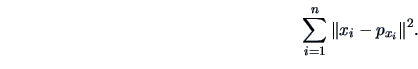
The question is how to project this
point cloud onto a space of lower dimension.
To begin consider the simplest
problem, namely finding a subspace of dimension
(considering each row).
The question is how to project this
point cloud onto a space of lower dimension.
To begin consider the simplest
problem, namely finding a subspace of dimension ![]() .
The problem boils down to finding a straight line
.
The problem boils down to finding a straight line ![]() through the origin.
The direction of this line can be defined by a unit
vector
through the origin.
The direction of this line can be defined by a unit
vector
![]() .
Hence, we are searching for the vector
.
Hence, we are searching for the vector ![]() which gives the ``best'' fit of the initial cloud of
which gives the ``best'' fit of the initial cloud of ![]() points.
The situation is depicted in Figure 8.3.
points.
The situation is depicted in Figure 8.3.
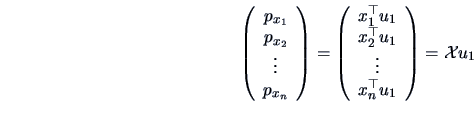
The representation of the ![]() -th individual
-th individual
![]() on this line is obtained by the projection of the
corresponding
point onto
on this line is obtained by the projection of the
corresponding
point onto ![]() , i.e., the projection point
, i.e., the projection point
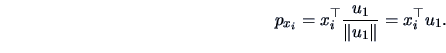
![]() . We know from (2.42) that
the coordinate of
. We know from (2.42) that
the coordinate of ![]() on
on ![]() is given by
is given by
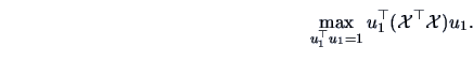
The solution is given by Theorem 2.5 (using
![]() and
and
![]() in the theorem).
in the theorem).
Note that if the data have been centered, i.e.,
![]() , then
, then
![]() , where
, where ![]() is the centered data matrix, and
is the centered data matrix, and
![]() is the covariance matrix.
Thus Theorem 8.1 says that we are searching for a maximum
of the quadratic form (8.3) w.r.t. the covariance matrix
is the covariance matrix.
Thus Theorem 8.1 says that we are searching for a maximum
of the quadratic form (8.3) w.r.t. the covariance matrix
![]() .
.
The coordinates of the ![]() individuals on
individuals on ![]() are given by
are given by ![]() .
.
![]() is called the first factorial
variable or the first factor and
is called the first factorial
variable or the first factor and ![]() the first factorial axis.
The
the first factorial axis.
The ![]() individuals,
individuals, ![]() , are now represented by a
new factorial variable
, are now represented by a
new factorial variable
![]() . This factorial variable is a linear
combination of the original variables
. This factorial variable is a linear
combination of the original variables
![]() whose coefficients are given
by the vector
whose coefficients are given
by the vector ![]() , i.e.,
, i.e.,
| (8.4) |
If we approximate the ![]() individuals by a plane (dimension 2),
it can be shown via Theorem 2.5 that this space contains
individuals by a plane (dimension 2),
it can be shown via Theorem 2.5 that this space contains
![]() .
The plane is determined by the best linear fit
(
.
The plane is determined by the best linear fit
(![]() ) and a unit vector
) and a unit vector ![]() orthogonal to
orthogonal to
![]() which maximizes the quadratic form
which maximizes the quadratic form
![]() under the constraints
under the constraints
The unit vector ![]() characterizes a second line,
characterizes a second line, ![]() ,
on which the points are projected.
The coordinates of the
,
on which the points are projected.
The coordinates of the ![]() individuals on
individuals on ![]() are given by
are given by
![]() . The variable
. The variable ![]() is called the
second factorial variable or the second factor.
The representation of the
is called the
second factorial variable or the second factor.
The representation of the ![]() individuals in
two-dimensional space (
individuals in
two-dimensional space (
![]() vs.
vs.
![]() )
is shown in Figure 8.4.
)
is shown in Figure 8.4.
In the case of ![]() dimensions the task is again to minimize
(8.2) but with projection points in a
dimensions the task is again to minimize
(8.2) but with projection points in a ![]() -dimensional
subspace.
Following the same argument as above, it can be shown
via Theorem 2.5 that this best
subspace is generated by
-dimensional
subspace.
Following the same argument as above, it can be shown
via Theorem 2.5 that this best
subspace is generated by
![]() , the
orthonormal
eigenvectors of
, the
orthonormal
eigenvectors of
![]() associated with the corresponding eigenvalues
associated with the corresponding eigenvalues
![]() .
The coordinates of the
.
The coordinates of the ![]() individuals on the
individuals on the ![]() -th factorial
axis,
-th factorial
axis, ![]() , are given by the
, are given by the ![]() -th factorial variable
-th factorial variable
![]() for
for
![]() .
Each factorial variable
.
Each factorial variable
![]() is a linear combination of the original variables
is a linear combination of the original variables
![]() whose coefficients are given by the elements of the
whose coefficients are given by the elements of the ![]() -th vector
-th vector
![]() .
.
![\includegraphics[width=1.4\defpicwidth]{fig353.ps}](mvahtmlimg2480.gif)
![\includegraphics[width=0.85\defpicwidth]{fig35z.ps}](mvahtmlimg2512.gif)