9.4 Asymptotic Properties of the PCs

In practice, PCs are computed from sample data. The following theorem yields results on the asymptotic distribution of the sample PCs.

THEOREM 9.4   Let $\Sigma > 0$ with distinct eigenvalues, and let $\data{U}\sim m^{-1} W_p(\Sigma ,m)$ with spectral decompositions $\Sigma =\Gamma \Lambda \Gamma ^{\top}$, and $\data{U}=\data{G}\data{L}\data{G}^{\top}$. Then

(a)

$\sqrt m (\ell -\lambda )\stackrel{\cal L}{\longrightarrow} N_p(0,2\Lambda ^2)$,
where $\ell =(\ell _1,\ldots ,\ell _p)^{\top}$ and $\lambda =(\lambda _1,\ldots ,\lambda _p)^{\top}$ are the diagonals of $\data{L}$ and $\Lambda$,

(b)

$\sqrt m(g_j-\gamma _j)\stackrel{\cal L}{\longrightarrow} N_p(0,\data{V}_j)$,
with $$\data{V}_j=\lambda _j\sum\limits_{k\neq j} \frac{\lambda _k}{(\lambda _k-\lambda _j)^2 }\gamma _k\gamma _k^{\top}$$,

(c)

$\mathop{\mathit{Cov}}(g_j,g_k) = \data{V}_{jk}$,
where the $(r,s)$-element of the matrix $\data{V}_{jk} (p\times p)$ is $$-\frac{\lambda _j\lambda _k\gamma _{rk}\gamma _{sj} } {[m(\lambda _j-\lambda _k)^2] }$$,

(d)

the elements in $\ell$ are asymptotically independent of the elements in $\data{G}$.

EXAMPLE 9.4   Since $n\data{S}\sim W_p(\Sigma ,n-1)$ if $X_1,\ldots,X_n$ are drawn from $N(\mu,\Sigma)$, we have that

$$\sqrt {n-1}(\ell _j-\lambda _j)\stackrel{\cal L}{\longrightarrow} N(0,2\lambda _j^2),\quad j=1,\ldots ,p.$$ (9.17)

Since the variance of (9.17) depends on the true mean $\lambda_j$ a log transformation is useful. Consider $f(\ell_j) = \log(\ell_j)$. Then $\frac{d}{d \ell_j}f\vert _{\ell_j = \lambda_j} = \frac{1}{\lambda_j}$ and by the Transformation Theorem 4.11 we have from (9.17) that

$$\sqrt{n-1} (\log \ell_j - \log \lambda_j) \longrightarrow N(0,2).$$ (9.18)

Hence,

$$\sqrt {\frac{n-1 }{2 }}\left (\log \ell _j-\log\lambda _j\right ) \stackrel{\cal L}{\longrightarrow} N(0,1)$$

and a two-sided confidence interval at the $1-\alpha =0.95$ significance level is given by

$$\log(\ell _j)-1.96\sqrt {\frac{2 }{n-1 }}\le \log\lambda _j\le \log(\ell _j)+1.96 \sqrt {\frac{2 }{n-1 }}.$$

In the bank data example we have that

$$\ell_1 =2.98.$$

Therefore,

$$\log(2.98)\pm 1.96 \sqrt {\frac{2 }{199 } }=\log(2.98)\pm 0.1965.$$

It can be concluded for the true eigenvalue that

$$P\left\{\lambda_1\in(2.448, 3.62)\right\}\approx 0.95.$$

Variance explained by the first $q$ PCs.

The variance explained by the first $q$ PCs is given by

$$\psi =\frac{\lambda _1+\cdots+\lambda _q } {\sum\limits^p_{j=1} \lambda _j}\cdotp$$

In practice this is estimated by

$$\widehat \psi =\frac{\ell _1+\cdots+\ell _q } {\sum\limits^p_{j=1}\ell _j }\cdotp$$

From Theorem 9.4 we know the distribution of $\sqrt {n-1}(\ell -\lambda )$. Since $\psi$ is a nonlinear function of $\lambda$, we can again apply the Transformation Theorem 4.11 to obtain that

$$\sqrt {n-1}(\widehat \psi -\psi )\stackrel{\cal L}{\longrightarrow} N(0,\data{D}^{\top}\data{V}\data{D})$$

where $\data{V} = 2\Lambda ^2$ (from Theorem 9.4) and $\data{D} = (d_1,\ldots ,d_p)^{\top}$ with

$$d_j=\frac{\partial \psi} {\partial \lambda_j } =\left\{ \beg... ...gma)} &\quad \textrm{ for } q+1 \le j\le p. \end{array}\right.$$

Given this result, the following theorem can be derived.

THEOREM 9.5  

$$\sqrt {n-1}(\widehat \psi -\psi )\stackrel{\cal L}{\longrightarrow} N(0,\omega^2),$$

where

$$\begin{eqnarray*} \omega^2 &=& \data{D}^{\top}\data{V}\data{D} = \frac{2} {\{\... ...athop{\hbox{tr}}(\Sigma )\}^2 } (\psi ^2-2\beta \psi +\beta ) \end{eqnarray*}$$

and

$$\beta = {\displaystyle \frac{\lambda ^2_1+\cdots+\lambda ^2_q } {\lambda ^2_1+\cdots+\lambda ^2_p } }.$$

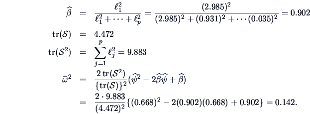
EXAMPLE 9.5   From Section 9.3 it is known that the first PC for the Swiss bank notes resolves 67% of the variation. It can be tested whether the true proportion is actually 75%. Computing

$$\begin{eqnarray*} \widehat\beta &=& \frac{\ell^2_1}{\ell^2_1+\cdots+\ell ^2_p } ... ...t 9.883 } {(4.472)^2}\{(0.668)^2-2(0.902)(0.668)+0.902\}=0.142. \end{eqnarray*}$$

Hence, a confidence interval at a significance of level $1-\alpha =$ 0.95 is given by

$$0.668\pm1.96\sqrt {\frac{0.142 }{199 }}=(0.615,0.720).$$

Clearly the hypothesis that $\psi =$ 75% can be rejected!

Summary

$\ast$

The eigenvalues $\ell_{j}$ and eigenvectors $g_{j}$ are asymptotically, normally distributed, in particular $\sqrt{n-1}(\ell-\lambda)\mathrel{\mathop{\longrightarrow}\limits_{}^{\cal L}} N_{p}(0,2\Lambda^2)$.

$\ast$

For the eigenvalues it holds that $\sqrt {\frac{n-1 }{2 }}\left (\log \ell _j-\log\lambda _j\right ) \stackrel{\cal L}{\longrightarrow} N(0,1)$.

$\ast$

Given an asymptotic, normal distribution approximate confidence intervals and tests can be constructed for the proportion of variance which is explained by the first $q$ PCs. The two-sided confidence interval at the $1-\alpha =0.95$ level is given by $\log(\ell _j)-1.96\sqrt {\frac{2 }{n-1 }}\le \log\lambda _j\le \log(\ell _j)+1.96 \sqrt {\frac{2 }{n-1 }}.$

$\ast$

It holds for $\widehat \psi$, the estimate of $\psi$ (the proportion of the variance explained by the first $q$ PCs) that $\sqrt {n-1}(\widehat \psi -\psi )\stackrel{\cal L}{\longrightarrow} N(0,\omega^2)$, where $\omega$ is given in Theorem 9.5.