When we want to study the properties of the obtained estimators,
it is convenient to distinguish between two categories of
properties: i) the small (or finite) sample properties, which are
valid whatever the sample size, and ii) the asymptotic properties,
which are associated with large samples, i.e., when ![]() tends to
tends to
![]() .
.
Given that, as we obtained in the previous section, the OLS and ML
estimates of ![]() lead to the same result, the following
properties refer to both. In order to derive these properties, and
on the basis of the classical assumptions, the vector of estimated
coefficients can be written in the following alternative form:
lead to the same result, the following
properties refer to both. In order to derive these properties, and
on the basis of the classical assumptions, the vector of estimated
coefficients can be written in the following alternative form:
The unbiasedness property of the estimators means that, if we have
many samples for the random variable and we calculate the
estimated value corresponding to each sample, the average of these
estimated values approaches the unknown parameter. Nevertheless,
we usually have only one sample (i.e, one realization of the
random variable), so we can not assure anything about the distance
between
![]() and
and ![]() . This fact leads us to employ
the concept of variance, or the variance-covariance matrix if we
have a vector of estimates. This concept measures the average
distance between the estimated value obtained from the only sample
we have and its expected value.
. This fact leads us to employ
the concept of variance, or the variance-covariance matrix if we
have a vector of estimates. This concept measures the average
distance between the estimated value obtained from the only sample
we have and its expected value.
From the previous argument we can deduce that, although the unbiasedness property is not sufficient in itself, it is the minimum requirement to be satisfied by an estimator.
The consideration of
![]() allows us to define
efficiency as a second finite sample property.
allows us to define
efficiency as a second finite sample property.
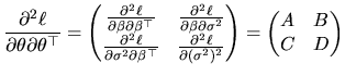
In order to study the efficiency property for the OLS and ML
estimates of ![]() , we begin by defining
, we begin by defining
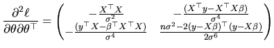
![]() , and the hessian
matrix is expressed as a partitioned matrix of the form:
, and the hessian
matrix is expressed as a partitioned matrix of the form:
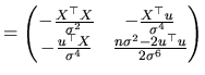
From (2.50) and (2.51), we have:
Following the Cramer-Rao inequality, ![]() constitutes the
lower bound for the variance-covariance matrix of any unbiased
estimator vector of the parameter vector
constitutes the
lower bound for the variance-covariance matrix of any unbiased
estimator vector of the parameter vector ![]() , while
, while ![]() is the corresponding bound for the variance of an unbiased
estimator of
is the corresponding bound for the variance of an unbiased
estimator of
![]() .
.
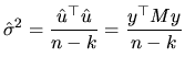
According to (2.56), we can conclude that
![]() (or
(or
![]() ), satisfies the efficiency
property, given that their variance-covariance matrix coincides
with
), satisfies the efficiency
property, given that their variance-covariance matrix coincides
with ![]() .
.
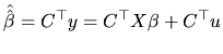
With this aim, we define
![]() as a family of linear
vectors of estimates of the parameter vector
as a family of linear
vectors of estimates of the parameter vector ![]() :
:
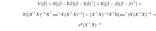
![$\displaystyle V(\hat{\hat{\beta}})=\textrm{E}[(\hat{\hat{\beta}}-\textrm{E}
\hat{\hat{\beta}})(\hat{\hat{\beta}}-\textrm{E}
\hat{\hat{\beta}})^{\top }]
$](xegbohtmlimg579.gif)
Taking into account (2.65) we have:
A general result matrix establishes that given any matrix P, then
![]() is a positive semidefinite matrix, so we can
conclude that
is a positive semidefinite matrix, so we can
conclude that
![]() is positive semidefinite. This
property means that the elements of its diagonal are non negative,
so we deduce for every
is positive semidefinite. This
property means that the elements of its diagonal are non negative,
so we deduce for every ![]() coefficient:
coefficient:
The set of results we have previously obtained, allows us to know
the probability distribution for
![]() (or
(or
![]() ). Given that these estimator vectors are linear
with respect to the
). Given that these estimator vectors are linear
with respect to the ![]() vector, and
vector, and ![]() having a normal
distribution, then:
having a normal
distribution, then:
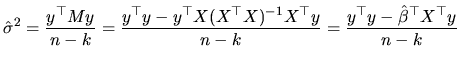
According to expressions (2.34) and (2.53),
the OLS and ML estimators of
![]() are different, despite
both being constructed through
are different, despite
both being constructed through
![]() . In
order to obtain their properties, it is convenient to express
. In
order to obtain their properties, it is convenient to express
![]() as a function of the disturbance of the
model. From the definition of
as a function of the disturbance of the
model. From the definition of ![]() in (2.26) we
obtain:
in (2.26) we
obtain:
Result (2.75), which means that ![]() is linear with
respect to
is linear with
respect to ![]() , can be extended in the following way:
, can be extended in the following way:
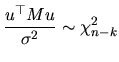
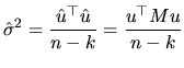
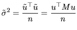
From (2.76), and under the earlier mentioned properties of
![]() , the sum of squared residuals can be written as a quadratic
form of the disturbance vector,
, the sum of squared residuals can be written as a quadratic
form of the disturbance vector,
Note that from (2.75), it is also possible to write
![]() as a quadratic form of
as a quadratic form of ![]() , yielding:
, yielding:
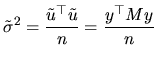
This expression for
![]() allows us to obtain
a very simple way to calculate the OLS or ML estimator of
allows us to obtain
a very simple way to calculate the OLS or ML estimator of
![]() . For example, for
. For example, for
![]() :
:
Having established these relations of interest, we now define the
properties of
![]() and
and
![]() :
:
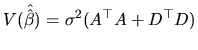
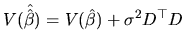
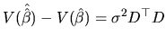
Nevertheless, given that
![]() is biased, this
estimator can not be efficient, so we focus on the study of such a
property for
is biased, this
estimator can not be efficient, so we focus on the study of such a
property for
![]() . With respect to the BLUE
property, neither
. With respect to the BLUE
property, neither
![]() nor
nor
![]() are
linear, so they can not be BLUE.
are
linear, so they can not be BLUE.
Finite sample properties try to study the behavior of an estimator under the assumption of having many samples, and consequently many estimators of the parameter of interest. Thus, the average of these estimators should approach the parameter value (unbiasedness) or the average distance to the parameter value should be the smallest possible (efficiency). However, in practice we have only one sample, and the asymptotic properties are established by keeping this fact in mind but assuming that the sample is large enough.
Specifically, the asymptotic properties study the behavior of the
estimators as ![]() increases; in this sense, an estimator which is
calculated for different sample sizes can be understood as a
sequence of random variables indexed by the sample sizes (for
example,
increases; in this sense, an estimator which is
calculated for different sample sizes can be understood as a
sequence of random variables indexed by the sample sizes (for
example, ![]() ). Two relevant aspects to analyze in this
sequence are
). Two relevant aspects to analyze in this
sequence are
![]() and
and
![]() .
.
A sequence of random variables ![]() is said
is said
![]() to a constant
to a constant ![]() or to another random variable
or to another random variable ![]() , if
, if
Result (2.91) implies that all the probability of
the distribution becomes concentrated at points close to ![]() .
Result (2.92) implies that the values that the
variable may take that are not far from z become more probable as
.
Result (2.92) implies that the values that the
variable may take that are not far from z become more probable as
![]() increases, and moreover, this probability tends to one.
increases, and moreover, this probability tends to one.
A second form of convergence is convergence in
distribution. If ![]() is a sequence of random variables with
cumulative distribution function (
is a sequence of random variables with
cumulative distribution function (![]() )
) ![]() , then the
sequence
, then the
sequence
![]() to a variable
to a variable ![]() with
with ![]()
![]() if
if
Having established these preliminary concepts, we now consider the following desirable asymptotic properties : asymptotic unbiasedness, consistency and asymptotic efficiency.
Note that the second part of (2.96) also means that
the possible bias of
![]() disappears as
disappears as ![]() increases, so we can deduce that an unbiased estimator is also an
asymptotic unbiased estimator.
increases, so we can deduce that an unbiased estimator is also an
asymptotic unbiased estimator.
The second definition is based on the convergence in distribution
of a sequence of random variables. According to this definition,
an estimator
![]() is asymptotically unbiased if
its asymptotic expectation, or expectation of its limit
distribution, is the parameter
is asymptotically unbiased if
its asymptotic expectation, or expectation of its limit
distribution, is the parameter ![]() . It is expressed as
follows:
. It is expressed as
follows:
Since this second definition requires knowing the limit distribution of the sequence of random variables, and this is not always easy to know, the first definition is very often used.
In our case, since
![]() and
and
![]() are unbiased,
it follows that they are asymptotically unbiased:
are unbiased,
it follows that they are asymptotically unbiased:
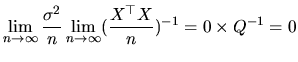
The simplest way of showing consistency consists of proving two sufficient conditions: i) the estimator must be asymptotically unbiased, and ii) its variance must converge to zero as n increases. These conditions are derived from the convergence in quadratic mean (or convergence in second moments), given that this concept of convergence implies convergence in probability (for a detailed study of the several modes of convergence and their relations, see Amemiya (1985), Spanos (1986) and White (1984)).
In our case, since the asymptotic unbiasedness of
![]() and
and
![]() has been shown earlier, we only have to prove
the second condition. In this sense, we calculate:
has been shown earlier, we only have to prove
the second condition. In this sense, we calculate:
where we have used the condition (2.6) included in
assumption 1. Thus, result (2.101) proves the
consistency of the OLS and ML estimators of the coefficient
vector. As we mentioned before, this means that all the
probability of the distribution of
![]() (or
(or ![]() )
becomes concentrated at points close to
)
becomes concentrated at points close to ![]() , as
, as ![]() increases.
increases.
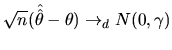
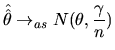
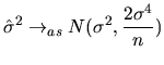
Suppose we have applied a CLT, and we have:
![$ \gamma=V_{as}[\sqrt{n}(\hat{\hat{\theta}}-\theta)]$](xegbohtmlimg656.gif) , that is
to say,
, that is
to say,  . This result allows us to
approach the limit distribution of
. This result allows us to
approach the limit distribution of
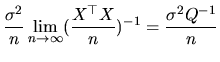
The second definition of asymptotic variance, which does not require using any limit distribution, is obtained as:
![$\displaystyle V_{as}(\hat{\beta})=\frac{1}{n}\lim_{n\rightarrow\infty}\textrm{E...
...trm{E}\hat{\beta}))((\hat{\beta}-\textrm{E}\hat{\beta})^{\top }\sqrt{n})]= \\
$](xegbohtmlimg663.gif)
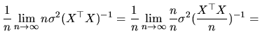
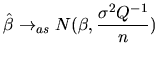
If we consider the first approach of the asymptotic variance, the use of a CLT (see Judge, Carter, Griffiths, Lutkepohl and Lee (1988)) yields:
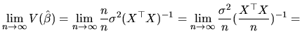
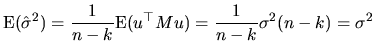
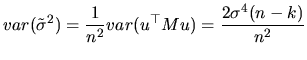
Finally, we should note that the finite sample efficiency implies
asymptotic efficiency, and we could have used this fact to
conclude the asymptotic efficiency of
![]() (or
(or
![]() ), given the results of subsection about their finite
sample properties.
), given the results of subsection about their finite
sample properties.
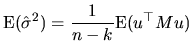
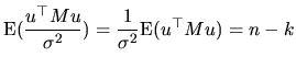
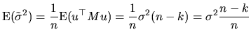
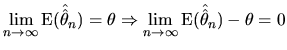
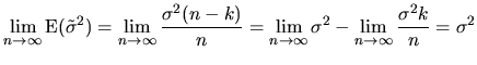
With respect to the ML estimator of
![]() , which does not
satisfy the finite sample unbiasedness (result
(2.87)), we must calculate its asymptotic
expectation. On the basis of the first definition of asymptotic
unbiasedness, presented in (2.96), we have:
, which does not
satisfy the finite sample unbiasedness (result
(2.87)), we must calculate its asymptotic
expectation. On the basis of the first definition of asymptotic
unbiasedness, presented in (2.96), we have:
| (2.117) |
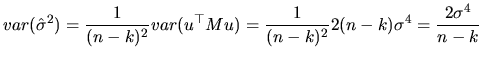
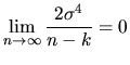
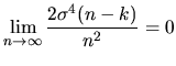
The second way to approach the asymptotic variance (see (2.104) ), leads to the following expressions:
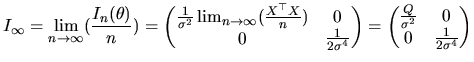
As we have seen in the previous section, the quantlet
 gls
allows us to estimate all the parameters of the MLRM. In addition,
if we want to estimate the variance-covariance matrix of
gls
allows us to estimate all the parameters of the MLRM. In addition,
if we want to estimate the variance-covariance matrix of
![]() , which is given by
, which is given by
![]() , we can use the following
quantlet
, we can use the following
quantlet
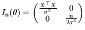
![$\displaystyle [I_{n}(\theta)]^{-1}= \begin{pmatrix}\sigma^{2}(X^{\top }X)^{-1} ...
...ma^{4}}{n} \end{pmatrix} = \begin{pmatrix}I^{11}& 0 \\ 0 & I^{22} \end{pmatrix}$](xegbohtmlimg572.gif)
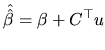
![$\displaystyle =\textrm{E}[(\hat{\hat{\beta}}-\beta)(\hat{\hat{\beta}}-\beta)^{\top }]= \textrm{E}[C^{\top }uu^{\top }C]=\sigma^{2}C^{\top }C$](xegbohtmlimg580.gif)


![$\displaystyle V_{as}(\hat{\hat{\theta}})=\frac{1}{n}\lim_{n\rightarrow\infty}\textrm{E}[\sqrt{n}(\hat{\hat{\theta}}-\textrm{E}(\hat{\hat{\theta}}))]^{2}$](xegbohtmlimg662.gif)
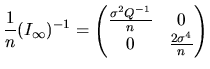
![$\displaystyle \frac{1}{n}(I_{\infty})^{-1}=\frac{1}{n}\left[\lim_{n\rightarrow\infty}(\frac{I_{n}(\theta)}{n})\right]^{-1}$](xegbohtmlimg670.gif)
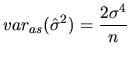
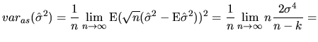
![$\displaystyle \frac{1}{n}\lim_{n\rightarrow\infty}\frac{2\sigma^{4}}{\frac{n-k}...
...a^{4}}{\lim_{n\rightarrow\infty}(1-\frac{k}{n})}\right] =\frac{1}{n}2\sigma^{4}$](xegbohtmlimg683.gif)
![$\displaystyle var_{as}(\tilde{\sigma}^{2})= \frac{1}{n}\lim_{n\rightarrow\infty...
...ma^{4}-\lim_{n\rightarrow\infty}\frac{2\sigma^{4}k}{n}]= \frac{1}{n}2\sigma^{4}$](xegbohtmlimg684.gif)