The binomial pricing model arises from discrete random walk models of the underlying asset. This method is only a reasonable approximation of the evolution of the stock prices when the number of trading intervals is large and the time between trades is small (Jarrow and Turnbull; 1996, pp. 213). It is particularly useful for pricing American options numerically, since it can deal with the possibility of early option exercise. An exact analytical solution with the Black-Scholes model for the American options is not possible, because of the complexity of the boundary conditions (see subsection 11.2.4).
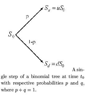
The binomial model breaks down the time to expiration of an option
into potentially very large number of time intervals, or steps. A
tree of stock prices is initially produced, moving forward from
the present to expiration. At each interval, the asset price ![]() can branch upwards to the value
can branch upwards to the value ![]() (Figure 11.3) or
downwards to the value
(Figure 11.3) or
downwards to the value ![]() , by an amount calculated using the
volatility and time to expiration. A binomial distribution of
prices, for the underlying asset is thus produced. The tree
represents all the possible paths that the stock price can take
during the life of the option.
, by an amount calculated using the
volatility and time to expiration. A binomial distribution of
prices, for the underlying asset is thus produced. The tree
represents all the possible paths that the stock price can take
during the life of the option.
At the end of the tree, i.e. at expiration of the option, the option values for each possible stock price are known, as they are equal to their intrinsic values. Assuming that the payoff function of the option is determined only by the value of the underlying asset at expiration, the model then works backwards through each time interval, calculating the option value at each step. The final step is at current time and stock price, where the theoretical fair value of the option is calculated. This recursive pricing procedure is based on the assumption of risk neutrality. In a risk neutral world all individuals require no compensation for risk, so that the option can be priced as though the underlying asset's expected return is risk-free.
The most popular binomial tree is that from Cox, Ross and Rubinstein (1979), also known as the Cox-Ross-Rubinstein (CRR) binomial tree. In this approach, the underlying asset evolves along a risk-neutral binomial tree with constant logarithmic price spacing, corresponding to constant volatility, as illustrated in Figure (11.4).
The CRR binomial tree is a discrete version of the Black-Scholes constant volatility process. Any higher multinomial tree, for example a trinomial tree, can used as a discrete development of the geometric Brownian motion. However, all of them converge, as the time interval tends to zero, to the same continuous constant volatility process. The CRR tree is discussed in subsection (11.3.2) and illustrated in the following computational examples in XploRe .
XploRe offers the folllowing quantlets to calculate European and American option prices with the Cox-Ross-Rubinstein binomial tree:
|
 asset
opens different interactive menus
for input parameters. It uses the quantlet
bitree
to price
European and American options.
asset
opens different interactive menus
for input parameters. It uses the quantlet
bitree
to price
European and American options.
The input parameter
![]() in the quantlets
asset
and
bitree
specifies the type of option. It has the value 1
for a call and 0 for a put.
in the quantlets
asset
and
bitree
specifies the type of option. It has the value 1
for a call and 0 for a put.
![]() is a scalar that specifies
the type of dividend payment(s): for
is a scalar that specifies
the type of dividend payment(s): for
![]() no dividend,
for
no dividend,
for
![]() a continuously paid dividend, for
a continuously paid dividend, for
![]() a dividend as a percentage of the value of the underlying asset
and for
a dividend as a percentage of the value of the underlying asset
and for
![]() a fixed dividend at the end of T is assumed.
If
a fixed dividend at the end of T is assumed.
If
![]() , then an exchange rate is assumed as underlying.
In this case,
, then an exchange rate is assumed as underlying.
In this case, ![]() is replaced by the exchange rate, i.e. the
domestic currency price of a unit foreign currency.
is replaced by the exchange rate, i.e. the
domestic currency price of a unit foreign currency.
When the quantlet
bitree
is used interactively, the first
five input parameters follow the usual notation: ![]() for the
price of the underlying asset,
for the
price of the underlying asset, ![]() for the strike price,
for the strike price,
![]() for the annualized risk-free interest rate in %,
for the annualized risk-free interest rate in %,
![]() for the annualized volatility in % and
for the annualized volatility in % and ![]() for time to expiration. The other parameters are:
for time to expiration. The other parameters are: ![]() for the
number of intervals in the tree,
for the
number of intervals in the tree, ![]() for the type of
option, which has the value 1 for a call (default) or 0 for a put.
The input parameter
for the type of
option, which has the value 1 for a call (default) or 0 for a put.
The input parameter
![]() specifies the type of
dividend payments. It has the values 0 to 4 for the same cases as
in
specifies the type of
dividend payments. It has the values 0 to 4 for the same cases as
in
![]() , with
, with
![]() as default. If
as default. If
![]() , then the value(s) of dividend(s)
must be specified in
, then the value(s) of dividend(s)
must be specified in ![]() . For more than one dividend
payment,
. For more than one dividend
payment, ![]() is a (m x 2) dimensional matrix, where the
first column contains the time points when dividends should be
paid and the second, the corresponding dividend values.
is a (m x 2) dimensional matrix, where the
first column contains the time points when dividends should be
paid and the second, the corresponding dividend values.
Both quantlets,
asset
and
bitree
output the tree
of possible prices of the underlying asset, which is contained in
a
![]() dimensional matrix
dimensional matrix ![]() , the tree of
option prices, which is contained in a
, the tree of
option prices, which is contained in a
![]() dimensional matrix
dimensional matrix ![]() and the price of the option
and the price of the option ![]() .
.
In the following example, the European put price on a dividend
paying underlying asset ![]() is computed through quantlet
betree
:
is computed through quantlet
betree
:
When binomial trees are used in practice, the life of the option
is typically divided into 30 or more time steps, of length ![]() . This computation can be easily carried out with
XploRe
.
With 30 time steps, 31 possible stock prices and
. This computation can be easily carried out with
XploRe
.
With 30 time steps, 31 possible stock prices and ![]() , or
about one billion, possible stock prices are considered. The asset
returns in one step of the tree,
, or
about one billion, possible stock prices are considered. The asset
returns in one step of the tree, ![]() and
and ![]() , are chosen to match
the stock price volatility. A popular way of doing this is by
setting
, are chosen to match
the stock price volatility. A popular way of doing this is by
setting
 |
(11.39) |
IBTcrr
calculates the price of a European option on a
non-dividend paying underlying asset.
![]() specifies the
number of intervals in the tree and
specifies the
number of intervals in the tree and
![]() is the length of
the discrete time interval.
is the length of
the discrete time interval.
![]() is a scalar, which has the
value
is a scalar, which has the
value ![]() for call and
for call and ![]() for put. The other parameters follow
the usual notation. The output window shows the calculated
European option price. The same price results when the quantlet
betree
is used. The last quantlet is recommended for
computation, since it yields not only the option price as in
IBTcrr
, but also the whole tree.
for put. The other parameters follow
the usual notation. The output window shows the calculated
European option price. The same price results when the quantlet
betree
is used. The last quantlet is recommended for
computation, since it yields not only the option price as in
IBTcrr
, but also the whole tree.
A second example illustrates how to price a European call with
IBTcrr
:
optstart
asks the user to specify the model, which will
compute the option price. It offers the Black-Scholes and the
MacMillan formulae as an analytical approach and the binomial tree
model as a numerical method. In the latter, the quantlet
bitree
is used for building the tree and pricing the
option.
The Cox, Ross and Rubinstein (CRR) binomial tree can be interpreted as a numerical procedure to solve the Black-Scholes equation. There are two main ideas underlying the tree. First, a continuous random walk (11.12) may be modelled by a discrete random walk with the following properties:
The second assumption underlying a binomial tree is that of a
risk-neutral world, i.e. the investor risk preferences are
irrelevant to option valuation. This has two implications. First,
the expected return from all traded securities is the risk-free
interest rate. This means that the drift term ![]() in the
stochastic differential equation for the asset return
(11.4) is replaced by the risk-free interest rate
in the
stochastic differential equation for the asset return
(11.4) is replaced by the risk-free interest rate ![]() whenever it appears
whenever it appears
Within this framework, the probabilities ![]() ,
, ![]() and the returns
and the returns ![]() ,
, ![]() should reflect the important statistical properties of the
continuous random walk (11.40), which means that they have
to insure that for
should reflect the important statistical properties of the
continuous random walk (11.40), which means that they have
to insure that for
![]() the underlying asset
the underlying asset
![]() follows the Brownian motion. In other words, the parameters
follows the Brownian motion. In other words, the parameters
![]() ,
, ![]() ,
, ![]() ,
, ![]() should give the correct values for the mean and
the variance of the underlying asset, i.e.
should give the correct values for the mean and
the variance of the underlying asset, i.e.
![]() , during a time interval
, during a time interval ![]() . Consequently, these
parameters must solve the following equations:
. Consequently, these
parameters must solve the following equations:
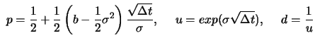
Substituting ![]() in (11.43) and (11.44), there are
three unknown parameters and two non-linear equations to solve. To
obtain a unique solution, a supplementary restriction for the
parameters is needed. Cox, Ross and Rubinstein (1979) chose the
restriction
in (11.43) and (11.44), there are
three unknown parameters and two non-linear equations to solve. To
obtain a unique solution, a supplementary restriction for the
parameters is needed. Cox, Ross and Rubinstein (1979) chose the
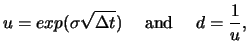
restriction ![]() , since it drastically simplifies the tree. At
time point
, since it drastically simplifies the tree. At
time point ![]() there are
only
there are
only
![]() possible nodes and
possible nodes and
| (11.45) |
Solving the equations (11.42), (11.43) and
(11.44) for ![]() ,
, ![]() , and
, and ![]() and neglecting the terms
smaller then
and neglecting the terms
smaller then ![]() results in:
results in:
The time steps are of equal length, so that the risk-neutral
probability ![]() as calculated by 11.46 is the same at each
node. The option price
as calculated by 11.46 is the same at each
node. The option price
![]() , at node
, at node ![]() and
time
and
time ![]() , is the expected payoff at
, is the expected payoff at ![]() discounted at the
risk-free interest rate:
discounted at the
risk-free interest rate:
| (11.47) |
When the underlying asset is a stock, which pays dividend(s), then the reduction of the stock prices by the dividend(s) amount must be considered. Details on the use of binomial trees for fixed or percentage dividend(s) are given in Franke et al. (2001, pp. 87).
In the case of an American put, or a European call on dividend
paying underlying asset, the option price will be checked at each
node to decide whether or not the early exercise would be optimal.
If the option is held until expiration, its value at the final
node is the same as for the European option. This is the case for
an American call, since there is always the chance that until
expiration the underlying price increases. Hence, the price of an
American call equals the price of its European counterpart.
![% latex2html id marker 54905
$\textstyle \parbox{5.95cm}{
{\includegraphics[wid...
...6\defpicwidth]{BT.ps}}
\caption{\small
CCR binomial tree. }\cite{de:ka:ch:96}}$](xlghtmlimg1074.gif)
![\includegraphics[width=1.5\defpicwidth]{binn.ps}](xlghtmlimg1128.gif)