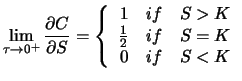
influence
from
the library
finance
in
XploRe
:
influence
from
the library
finance
in
XploRe
:
The Black-Scholes formula for non-dividend paying underlying
assets (11.10) show that there are essentially five
parameters, which determine the option price: the current level of
the underlying asset ![]() , the strike price
, the strike price ![]() , the continuously
compounded risk-free interest rate
, the continuously
compounded risk-free interest rate ![]() , the time to expiration
, the time to expiration
![]() and the instantaneous standard deviation
and the instantaneous standard deviation ![]() of the
underlying. The influence of these parameters on the option price
can be investigated by using the quantlet
influence
from
the library
finance
in
XploRe
:
of the
underlying. The influence of these parameters on the option price
can be investigated by using the quantlet
influence
from
the library
finance
in
XploRe
:
greeks
.
greeks
is specified in
The output is a two dimensional plot, which shows the dependence
of the option price (when the quantlet
influence
is used)
or of its sensitivity (when the quantlet
greeks
is used)
on the specified parameter. If an additional parameter is
specified in ![]() , a three dimensional plot with both
parameters as explanatory variables is produced.
, a three dimensional plot with both
parameters as explanatory variables is produced.
For graphical representation, the option price is computed within
30 discrete intervals of the explanatory variable(s). This is done
mainly in two steps. Firstly, the quantlet
asset
is used
to create a discrete grid of 31 points. To achieve this, the
lowest and highest bounds for the parameter(s) are requested. The
highest bound must be inputed into ![]() (and into
(and into ![]() in the case of two exploratory variables). The specified input
value of the exploratory variable(s) is considered as the lowest
bound. When both quantlets
influence
and
greeks
are used interactively, the user can freely decide which bound
values to apply. Secondly, the option price is computed for each
of the 31 different grid points using the Black-Scholes Formula.
The results are presented in a two dimensional, or for two
exploratory variables, in a three dimensional plot.
in the case of two exploratory variables). The specified input
value of the exploratory variable(s) is considered as the lowest
bound. When both quantlets
influence
and
greeks
are used interactively, the user can freely decide which bound
values to apply. Secondly, the option price is computed for each
of the 31 different grid points using the Black-Scholes Formula.
The results are presented in a two dimensional, or for two
exploratory variables, in a three dimensional plot.
In the following, the sensitivity of the option price with respect
to changes in one of the five parameters is analyzed: ![]() ,
,
![]() ,
, ![]() ,
, ![]() and
and
![]() . Details on these
sensitivities can be found in different financial sources, e.g. in
the e-book
Statistics of Financial Markets, ch. 7.3.
.
. Details on these
sensitivities can be found in different financial sources, e.g. in
the e-book
Statistics of Financial Markets, ch. 7.3.
.
The following theoretical descriptions are based on
Franke et al. (2001), Gibson (1991), Hull (2000), Kwock (1998) and Tompkinks (1994). To
demonstrate how the option price and its sensitivity relates to
the changes in the parameters above, the quantlets
influence
and
greeks
are used.
The delta (![]() ) of a derivative security is defined as the
rate of change of its price with respect to the price of the
underlying asset. It is the slope of the curve that relates the
derivative security price
) of a derivative security is defined as the
rate of change of its price with respect to the price of the
underlying asset. It is the slope of the curve that relates the
derivative security price ![]() to the price of the underlying
to the price of the underlying ![]() :
:

Delta plays a crucial role in portfolio hedging. In the derivation
of the Black-Scholes equation a covered call position is
maintained by creating a risk-free portfolio, where the writer of
a call sells one unit of the call and buys ![]() units of the
underlying.
units of the
underlying.
The delta of a call (![]() ) is always positive, as an
increase in the asset price will increase the probability of a
positive payoff at expiration resulting in a higher value. On the
other hand, there is a negative relationship between the put price
and the underlying asset price, as an increase in the asset price,
will reduce the put's current exercise value
) is always positive, as an
increase in the asset price will increase the probability of a
positive payoff at expiration resulting in a higher value. On the
other hand, there is a negative relationship between the put price
and the underlying asset price, as an increase in the asset price,
will reduce the put's current exercise value
![]() and therefore the put's price
will decrease. This explains a negative
and therefore the put's price
will decrease. This explains a negative ![]() as given in
(11.50).
as given in
(11.50).
When the price of the underlying asset changes, put and call
option values move in opposite directions, since
![]() and
and
![]() . However, the
absolute changes in their prices will never exceed those of the
underlying asset.
. However, the
absolute changes in their prices will never exceed those of the
underlying asset.
![]() of a European call on a non-dividend paying underlying
asset can be easily derived from the Black-Scholes formula
(11.10):
of a European call on a non-dividend paying underlying
asset can be easily derived from the Black-Scholes formula
(11.10):
In the following, it is shown through examples how the option price and its delta is calculated and plotted as a function of the underlying asset.
library("finance")

S=230 		; (spot) price of the underlying

K=210 		; exercise price

r=5 		; the annualized risk-free interest rate in %

sigma=25 		; annualized volatility  in %

tau=0.5 		; annualized time to expiration

carry=5 		; cost of carry

opt=1 		; call

v1=1 		; spot price as an explanatory variable

ub1=400 		; highest bound of the spot price

influence(S,K,r,sigma,tau,carry,opt,v1,ub1)


pdr=1 		; delta of the call

greeks(S,K,r,sigma,tau,carry,opt,pdr,v1,ub1)
The computation yields a (31x2) dimensional matrix with the
prices of the underlying asset in the first column. The second
column contains the respective call prices (for the quantlet
influence
), or the values of ![]() (for the quantlet
greeks
).
(for the quantlet
greeks
).
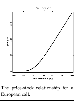
The two dimensional plot (Figure 11.6) displays a positive
relationship between the call price and the underlying, which
supports the theoretical results from (11.49). Note, for
explanation purposes the underlying ranges from 100 to 400. This
is achieved through running the quantlets
influence
and
greeks
once again and specifing interactively the
parameters with the same values, as in the example above.
Figure 11.7 shows that ![]() is an increasing
function of
is an increasing
function of ![]() . This result is not surprising, since
. This result is not surprising, since
![]() is always positive. It
follows that the call price is an increasing convex function of
the underlying price (see subsection 11.4.3 for further
details on convexity).
is always positive. It
follows that the call price is an increasing convex function of
the underlying price (see subsection 11.4.3 for further
details on convexity).
The fact that the delta changes as the underlying price changes, means that the delta provides only instantaneous information. To remain perfectly risk-free, a hedged position in options may have to be revised continuously. The delta-hedge frequency, depends on the derivative of the delta with respect to the price of the underlying, commonly referred to as the gamma. For detailed explanations and examples on gamma see subsection 11.4.3.
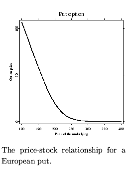
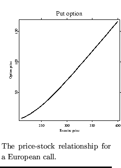
In a second example the same procedure is repeated for a put option:
The outputs are presented in Figure (11.8) and Figure
(11.9) respectively. Figure (11.9) shows that
![]() is an increasing function of the asset price
is an increasing function of the asset price ![]() , i.e.
the put's price decreases at an increasing rate, when the price of
the underlying asset increases. In other words, the put's price is
a decreasing convex function of the price of the underlying asset.
, i.e.
the put's price decreases at an increasing rate, when the price of
the underlying asset increases. In other words, the put's price is
a decreasing convex function of the price of the underlying asset.
Both call and put deltas are functions of ![]() and
and ![]() . It can
be shown that
. It can
be shown that
At expiration, delta has different asymptotic limits depending on
whether the option is in-the-money ![]() , at-the-money
, at-the-money ![]() ,
or out-of-the-money
,
or out-of-the-money ![]() . For options deep in-the-money,
. For options deep in-the-money,
![]() converges to one. In other words, since the option will
be exercised at expiration, the writer of the call should hold the
asset to hedge the risk. For deep out-of-the-money, the call will
not be exercised and the writer no longer needs to hold the asset.
Consequently,
converges to one. In other words, since the option will
be exercised at expiration, the writer of the call should hold the
asset to hedge the risk. For deep out-of-the-money, the call will
not be exercised and the writer no longer needs to hold the asset.
Consequently, ![]() will then converge to zero. Hence at
expiration, the option will have either a slope of zero (if
out-of-the-money) or one (if in-the-money).
will then converge to zero. Hence at
expiration, the option will have either a slope of zero (if
out-of-the-money) or one (if in-the-money).
It can be surmised that the at-the-money option, which lies in the
middle between these extremes, might have a slope of ![]() .
Therefore any time before expiration an out-of-the-money option
will have a delta between 0 and
.
Therefore any time before expiration an out-of-the-money option
will have a delta between 0 and ![]() , and in-the money option
will have a delta between
, and in-the money option
will have a delta between ![]() and
and ![]() . For example, this can be
seen for a call option with six months prior to expiration in
Figure 11.7. The "S" shaped curve indicates how the
exposure of the call option relative to the underlying asset has a
limit loss when the price of the underlying asset falls, and
assumes full exposure when the underlying price rises.
. For example, this can be
seen for a call option with six months prior to expiration in
Figure 11.7. The "S" shaped curve indicates how the
exposure of the call option relative to the underlying asset has a
limit loss when the price of the underlying asset falls, and
assumes full exposure when the underlying price rises.
Alternative ways to think about delta, as a measure of relative risk of the option to the underlying market, or as the probability of exercise, are explained in Tompkinks (1994, pp. 57-65).
greeks
() computes ![]() and displays it as a function
of
and displays it as a function
of ![]() and
and ![]() (Figure 11.10). The input parameters are
given interactively. The plot supports the relationship mentioned
above.
(Figure 11.10). The input parameters are
given interactively. The plot supports the relationship mentioned
above.
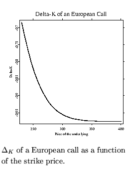
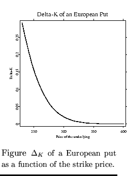
For most options the strike price is fixed, but some option-like
securities, such as convertible bonds, can have a variable
"strike" price. In this case the price change of the derivative
security ![]() with respect to the strike price
with respect to the strike price ![]()

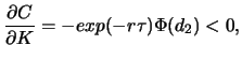
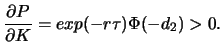
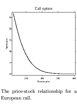
may be appropriate. The higher the strike price, the less valuable a call option is, since the strike price represents a higher cost of exercising the call and thereby purchasing the stock. In contrast, the higher the exercise price of a put, the higher its price will be. The Black-Scholes formula clearly confirms these relationships:
In the following example, the quantlet
influence
displays
the relationship between the option price and the strike price for
a European call (Figure 11.11) and a European put
(Figure 11.13). The quantlet
greeks
is used to plot
the respective deltas of the strike (Figure 11.12 and
11.14).
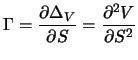
The option gamma (![]() ) is defined as the derivative of delta
(
) is defined as the derivative of delta
(![]() ) with respect to the underlying asset price
) with respect to the underlying asset price ![]() :
:
It represents the change in the curvature of the option at
different values of ![]() and is therefore also known as convexity.
The increments of gamma are often referred to as the number of
deltas that will change when the underlying asset price changes by
one tick. By definition, the higher the gamma value is, the more
the delta will change when the underlying market price changes.
and is therefore also known as convexity.
The increments of gamma are often referred to as the number of
deltas that will change when the underlying asset price changes by
one tick. By definition, the higher the gamma value is, the more
the delta will change when the underlying market price changes.
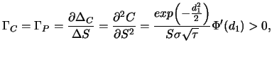
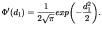
The gamma of a long European call and a long European put on a non-dividend paying underlying asset is
with ![]() defined as in equation (11.10) and
defined as in equation (11.10) and
![]() defined as
defined as
A positive gamma as in (11.53) and (11.54) means that changes in the amount of delta have the same direction as changes in the underlying market. This explains why for any European vanilla call or put option, the curves of the option price functions are convex with respect to the asset price (Figure 11.7 and 11.9).
With gamma being positive, the buyers of the options gain from movements in the price of the underlying assets. For this reason, holders of the options are often referred to as being "long gamma". For sellers of the options, the gamma exposure is exactly opposite to that of buyers of options. Those who sells options can be hurt when gamma is high and the underlying market price moves. Therefore they are often referred to as "short gamma".
When the curvature of the option value is small, its gamma has a low value. A low value of gamma implies that delta changes slowly with the asset price and so adjustments required to keep a portfolio delta neutral can be made less frequently. When gamma is high, in absolute terms, delta is highly sensitive to the price of the underlying asset. It is then quite risky to leave a delta-neutral portfolio unchanged for any remaining length of time.
Intuitively, gamma jointly measures how close the current market
is to the option strike price and how close the option is to
expiration (Tompkinks; 1994, pp. 67). The closer the market price is to
the strike price and the closer the option is to expiration, the
higher the gamma will be. This is illustrated in
Figure (11.15) for a European call option with ![]() ,
, ![]() ,
, ![]() ,
,
![]() ,
,
![]() and
and
![]() . The computation is
done interactively by using the quantlet
greeks
().
. The computation is
done interactively by using the quantlet
greeks
().
When the option is at-the-money (![]() ) with one minute
remaining until expiration, it has the highest possible gamma
value of
) with one minute
remaining until expiration, it has the highest possible gamma
value of ![]() . The reason for this, is that if the underlying
asset price moves the tiniest increment up, the option will then
be in-the-money with a delta of
. The reason for this, is that if the underlying
asset price moves the tiniest increment up, the option will then
be in-the-money with a delta of ![]() (Figure 11.15).
If on the other hand, the underlying asset price falls by an
infinitesimally small amount, the option will then be
out-of-the-money with a delta of zero.
(Figure 11.15).
If on the other hand, the underlying asset price falls by an
infinitesimally small amount, the option will then be
out-of-the-money with a delta of zero.
More moving away from this extreme situation, where the option is at-the-money at expiration, then the lower the gearing effect of the option will be, hence the lower the gamma. The larger the difference between the current underlying asset price and the options's strike price, the less is the time value of the option and the lower the gamma. Additionally, an option with more time remaining until expiration will have a lower gamma (Figure 11.15).
So far the speed (delta) and acceleration (gamma) features of options over the underlying market price have been examined. In the following the other factors are discussed, the most important being volatility.
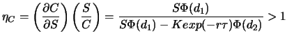
The change in the option price with respect to the change in
implied volatility (section 11.5) is called vega. It is a
measure of the option exposure to changes in implied volatility
within the option market (Tompkinks; 1994, pp. 69). The vega of a
European vanilla call ![]() and put
and put ![]() on
non-dividend paying underlying asset can be derived from the
Black-Scholes formula:
on
non-dividend paying underlying asset can be derived from the
Black-Scholes formula:
When the volatility rises, the option's set of favorable outcomes will also rise. As a result, the chances are higher for the option to be either deeper in-the-money or deeper out-of-the-money at expiration. Since the option bears no downside risk, there is no penalty when the option expires deeper out-of-the-money, but a higher payoff when it expires deeper in-the-money. Due to this antisymmetric payoff structure, the vegas for long options are positive, i.e. for the option buyer, the exposure to changes in implied volatility is positive and consequently the vega is positive. By symmetry, the option writer benefits from a decrease in implied volatility and therefore has vega negative exposure.
Using interactive menus in the quantlet
greeks
(), the vega
of a European call option is presented as a function of the
underlying asset and of time to expiration
(Figure 11.16). For at-the-money options, the longer
the time to expiration, the higher the sensitivity of the option
to the changes in volatility, and hence the higher the vega. In
other words, whereas gamma of an at-the-money option increases as
the expiration date approaches (see Figure 11.15), the
reverse is true for vega.
Eta (![]() ) of a derivative security defines the elasticity of
its price
) of a derivative security defines the elasticity of
its price ![]() with respect to the underlying price
with respect to the underlying price ![]() :
:
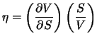
This elasticity parameter measures the percentage change in
security price for a unit percentage change in the asset price.
The elasticity of a European vanilla call (![]() ) on
non-dividend paying underlying asset is found to be:
) on
non-dividend paying underlying asset is found to be:
Equation (11.58) implies that a call option is riskier than
the underlying asset in terms of change in percentage. It can be
shown that the elasticity is high when the asset price is low
(out-of-the-money), and it decreases monotonously with the price
of the underlying asset (Kwock; 1998, pp. 57). For sufficiently
large values of ![]() ,
, ![]() converges to one, as
converges to one, as ![]() approaches
approaches
![]() when
when ![]() tends to infinity. This relationship can be seen in
Figure (11.17), which plots the elasticity of a European
call from the following example:
tends to infinity. This relationship can be seen in
Figure (11.17), which plots the elasticity of a European
call from the following example:
library("finance")
 greeks(230,210,5,25,0.5,5,1,3,2,400) ; call
The elasticity of a European put price (
For both put and call options, their elasticities increase in absolute value when the corresponding options become more out-of-the-money and move closer to expiration (Kwock; 1998, pp. 57).
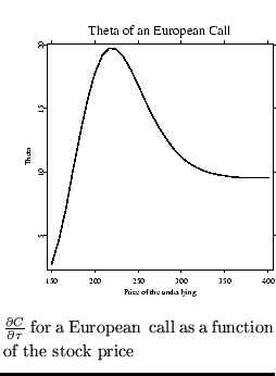
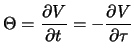
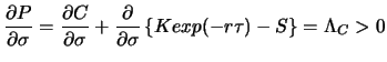
Theta (![]() ) of a derivative security is defined as the rate
of change of its price
) of a derivative security is defined as the rate
of change of its price ![]() with respect to time
with respect to time ![]() with all other
factors remaining constant:
with all other
factors remaining constant:
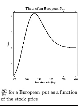
![]() for a European call and a
European put is computed in
XploRe
, by specifying the input
parameters interactively. The plots are shown in
Figure (11.18) and (11.19). The underlying
price
for a European call and a
European put is computed in
XploRe
, by specifying the input
parameters interactively. The plots are shown in
Figure (11.18) and (11.19). The underlying
price ![]() ranges from 150 to 400. The values of the other input
parameters are
ranges from 150 to 400. The values of the other input
parameters are
![]() ,
,
![]() ,
,
![]() ,
,
![]() ,
,
![]() .
.
greeks
considers
The theta of a European call (Figure 11.18) has its
greatest absolute value when the call option is at-the-money, as
it may become in-the-money or out-of-the-money soon thereafter. It
has a small absolute value when the option is sufficiently
out-of-the-money, as it will be highly unlikely for the option to
become in-the-money later on. It tends asymptotically to
![]() when the asset price is sufficiently
high.
when the asset price is sufficiently
high.
The theta of a European put (Figure 11.19) can be any
sign, depending on the relative magnitudes of the two terms, which
have opposite signs in (11.61). When the European put is
deep in-the-money, S assumes a small value, so that
![]() tends to one. The second term
tends to one. The second term
![]() is then greater than the
first
is then greater than the
first
![]() . In this
case,
. In this
case,
![]() is negative and the theta
as defined in (11.61) is positive. When the option is
at-the-money or out-of-the-money,
is negative and the theta
as defined in (11.61) is positive. When the option is
at-the-money or out-of-the-money,
![]() is typically positive and hence the theta of a European put
is negative, as the longer the time to expiration, the higher the
chances of positive outcomes.
is typically positive and hence the theta of a European put
is negative, as the longer the time to expiration, the higher the
chances of positive outcomes.
Note, the ambiguous relationship between a put's price and time to expiration does not hold for American options. An American call or put will always show a positive relationship between its price and time to expiration, which corresponds to a negative theta. When the time to expiration is prolonged, an American option has therefore the additional right to be exercised in the prolonged time interval and consequently has a higher value.
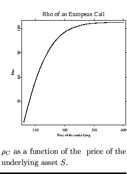
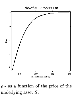
The Rho (![]() ) of a derivative security is defined as the rate
of change of derivative price
) of a derivative security is defined as the rate
of change of derivative price ![]() with respect to the interest
rate
with respect to the interest
rate ![]() :
:

The following example calculates ![]() and
and ![]() and plots
them against the underlying asset price
and plots
them against the underlying asset price ![]() (Figure 11.20
and 11.21).
(Figure 11.20
and 11.21).
library("finance")
 greeks(230,210,5,25,0.5,5,1,7,1,400) ; call
 greeks(230,210,5,25,0.5,5,0,7,1,400) ; put
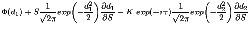
![$\displaystyle \Phi(d_1)+ \frac{1}{\sigma\sqrt{2\pi\tau}}
\left[exp{\left(-\frac...
...t(r\tau+ln\frac{S}{K}\right)\right\}}
exp{\left(-\frac{d^2_2}{2}\right)}\right]$](xlghtmlimg1148.gif)


![\includegraphics[width=1\defpicwidth]{greeksDeltaSta.ps}](xlghtmlimg1162.gif)
![\includegraphics[width=1\defpicwidth]{greeksGammaSta2.ps}](xlghtmlimg1185.gif)
![\includegraphics[width=1\defpicwidth]{greeksVegaSta1.ps}](xlghtmlimg1195.gif)
![\includegraphics[width=0.8\defpicwidth]{greeksEtaSa.ps}](xlghtmlimg1199.gif)