Let us first study the linear regression model
![]() assuming
assuming
![]() . Unless said otherwise, we consider here only one dependent
variable
. Unless said otherwise, we consider here only one dependent
variable ![]() . The unknown vector
. The unknown vector
![]() is to be estimated given observations
is to be estimated given observations
![]() and
and
![]() of random variables
of random variables ![]() and
and
![]() ; let us denote
; let us denote
![]() and let
and let
![]() be the
be the ![]() th column of
th column of
![]() . Thus,
the linear regression model can be written in terms of observations as
. Thus,
the linear regression model can be written in terms of observations as
Section 8.1.1 summarizes how to estimate the model (8.1) by the method of least squares. Later, we specify what ill-conditioning and multicollinearity are in Sect. 8.1.2 and discuss methods dealing with it in Sects. 8.1.3-8.1.9.
Let us first review the least squares estimation and its main properties to facilitate easier understanding of the fitting procedures discussed further. For a detailed overview of linear regression modeling see [75].
The least squares (LS)
approach to the estimation of (8.1) searches an estimate
![]() of unknown parameters
of unknown parameters
![]() by minimizing the sum of squared
differences between the observed values
by minimizing the sum of squared
differences between the observed values ![]() and the predicted ones
and the predicted ones
![]() .
.
This differentiable problem can be expressed as minimization of
Assumethat
![]() ,
,
![]() , and
, and
![]() is non-singular. Let
is non-singular. Let
![]() , where
, where
![]() is a
is a
![]() matrix orthogonal to
matrix orthogonal to
![]() ,
,
![]() . Then
. Then
![]() is a positive definite
matrix for any
is a positive definite
matrix for any
![]() .
.
Finally, the LS estimate actually coincides with the maximum
likelihood estimates provided that random errors
![]() are normally
distributed (in addition to the assumptions of Theorem 1)
and shares then the asymptotic properties of the maximum likelihood
estimation (see [4]).
are normally
distributed (in addition to the assumptions of Theorem 1)
and shares then the asymptotic properties of the maximum likelihood
estimation (see [4]).
The LS estimate
![]() can be and often
is found by directly solving the system of linear
equations (8.3) or evaluating formula (8.4),
which involves a matrix inversion. Both direct and iterative methods
for solving systems of linear equations are presented in
Chap. II.4. Although this straightforward computation may work well
for many regression problems, it often leads to an unnecessary loss of
precision, see [68]. Additionally, it is not very
suitable if the matrix
can be and often
is found by directly solving the system of linear
equations (8.3) or evaluating formula (8.4),
which involves a matrix inversion. Both direct and iterative methods
for solving systems of linear equations are presented in
Chap. II.4. Although this straightforward computation may work well
for many regression problems, it often leads to an unnecessary loss of
precision, see [68]. Additionally, it is not very
suitable if the matrix
![]() is ill-conditioned
(a regression problem is called ill-conditioned if a small change in
data causes large changes in estimates) or nearly singular
(multicollinearity) because it is not numerically stable. Being
concerned mainly about statistical consequences of multicollinearity,
the numerical issues regarding the identification and treatment of
ill-conditioned regression models are beyond the scope of this
contribution. Let us refer an interested reader
[6,13,68,92] and [99].
is ill-conditioned
(a regression problem is called ill-conditioned if a small change in
data causes large changes in estimates) or nearly singular
(multicollinearity) because it is not numerically stable. Being
concerned mainly about statistical consequences of multicollinearity,
the numerical issues regarding the identification and treatment of
ill-conditioned regression models are beyond the scope of this
contribution. Let us refer an interested reader
[6,13,68,92] and [99].
Let us now briefly review a class of numerically more stable
algorithms for the LS minimization.
They are based on orthogonal transformations. Assuming a matrix
![]() is an orthonormal matrix,
is an orthonormal matrix,
![]() ,
,
 |
Linear regression modeling does not naturally consist only of
obtaining a point estimate
![]() . One
needs to measure the variance of the estimates in order to construct
confidence intervals or test hypotheses. Additionally, one should
assess the quality of the regression fit. Most such measures are based
on regression residuals
. One
needs to measure the variance of the estimates in order to construct
confidence intervals or test hypotheses. Additionally, one should
assess the quality of the regression fit. Most such measures are based
on regression residuals
![]() . We briefly review the most important
regression statistics, and next, indicate how it is possible to
compute them if the LS regression is estimated by means of some
orthogonalization procedure described in the previous paragraph.
. We briefly review the most important
regression statistics, and next, indicate how it is possible to
compute them if the LS regression is estimated by means of some
orthogonalization procedure described in the previous paragraph.
The most important measures used in statistics to assess model fit and
inference are the total sum of squares
![]() ,
where
,
where
![]() , the residual sum of squares
, the residual sum of squares
![]() , and the complementary
regression sum of squares
, and the complementary
regression sum of squares
![]() . Using these quantities, the regression fit
can be evaluated; for example, the coefficient of determination
. Using these quantities, the regression fit
can be evaluated; for example, the coefficient of determination
![]() as well as many information criteria (modified
as well as many information criteria (modified
![]() , Mallows and Akaike criteria, etc.; see
Sect. 8.1.3). Additionally, they can be used to compute the
variance of the estimates in simple cases. The variance of the
estimates can be estimated by
, Mallows and Akaike criteria, etc.; see
Sect. 8.1.3). Additionally, they can be used to compute the
variance of the estimates in simple cases. The variance of the
estimates can be estimated by
Let us now describe how one computes these quantities if a numerically
stable procedure based on the orthonormalization of normal equations
is used. Let us assume we already constructed a QR decomposition of
![]() . Thus,
. Thus,
![]() and
and
![]() .
.
![]() can be
computed as
can be
computed as
 |
||
 |
Let us assume that the design matrix
![]() fixed. We talk about
multicollinearity when there is a linear dependence among the
variables in regression, that is, the columns of
fixed. We talk about
multicollinearity when there is a linear dependence among the
variables in regression, that is, the columns of
![]() .
.
The exact multicollinearity (also referred to as reduced-rank data) is
relatively rare in linear regression models unless the number of
explanatory variables is very large or even larger than the number of
observations, ![]() . This happens often in agriculture,
chemometrics, sociology, and so on. For example, [68]
uses data on the absorbances of infra-red rays at many different
wavelength by chopped meat, whereby the aim is to determine the
moisture, fat, and protein content of the meat as a function of these
absorbances. The study employs measurements at
. This happens often in agriculture,
chemometrics, sociology, and so on. For example, [68]
uses data on the absorbances of infra-red rays at many different
wavelength by chopped meat, whereby the aim is to determine the
moisture, fat, and protein content of the meat as a function of these
absorbances. The study employs measurements at ![]() wavelengths from
wavelengths from
![]() nm to
nm to
![]() nm, which gives rise to many
possibly correlated variables.
nm, which gives rise to many
possibly correlated variables.
When the number ![]() of variables is small compared to the sample size
of variables is small compared to the sample size
![]() , near multicollinearity
is more likely to occur: there are some real constants
, near multicollinearity
is more likely to occur: there are some real constants
![]() such that
such that
![]() and
and
![]() , where
, where ![]() denotes approximate
equality. The multicollinearity in data does not have to arise only
as a result of highly correlated variables (e.g., more measurements of
the same characteristic by different sensors or methods), which by
definition occurs in all applications where there are more variables
than observations, but it could also result from the lack of
information and variability in data.
denotes approximate
equality. The multicollinearity in data does not have to arise only
as a result of highly correlated variables (e.g., more measurements of
the same characteristic by different sensors or methods), which by
definition occurs in all applications where there are more variables
than observations, but it could also result from the lack of
information and variability in data.
Whereas the exact multicollinearity
implies that
![]() is singular and the LS estimator is not
identified, the near multicollinearity
permits non-singular matrix
is singular and the LS estimator is not
identified, the near multicollinearity
permits non-singular matrix
![]() . The eigenvalues
. The eigenvalues
![]() of matrix
of matrix
![]() can
give some indication concerning multicollinearity: if the smallest
eigenvalue
can
give some indication concerning multicollinearity: if the smallest
eigenvalue ![]() equals zero, the matrix is singular and data
are exactly multicollinear; if
equals zero, the matrix is singular and data
are exactly multicollinear; if ![]() is close to zero, near
multicollinearity is present in data. Since measures based on
eigenvalues depend on the parametrization of the model, they are not
necessarily optimal and it is often easier to detect multicollinearity
by looking at LS estimates and their behavior as discussed in next
paragraph. See [13] and [59] for more details on
detection and treatment of ill-conditioned problems. (Nearly singular
matrices are dealt with also in numerical mathematics. To measure near
singularity, numerical mathematics uses conditioning numbers
is close to zero, near
multicollinearity is present in data. Since measures based on
eigenvalues depend on the parametrization of the model, they are not
necessarily optimal and it is often easier to detect multicollinearity
by looking at LS estimates and their behavior as discussed in next
paragraph. See [13] and [59] for more details on
detection and treatment of ill-conditioned problems. (Nearly singular
matrices are dealt with also in numerical mathematics. To measure near
singularity, numerical mathematics uses conditioning numbers
![]() , which converge to infinity for singular
matrices, that is, as
, which converge to infinity for singular
matrices, that is, as
![]() . Matrices with very large
conditioning numbers are called ill-conditioned.)
. Matrices with very large
conditioning numbers are called ill-conditioned.)
The multicollinearity has important implications for LS.
In the case of exact multicollinearity, matrix
![]() does
not have a full rank, hence the solution of the normal equations is
not unique and the LS estimate
does
not have a full rank, hence the solution of the normal equations is
not unique and the LS estimate
![]() is not identified. One has to
introduce additional restrictions to identify the LS estimate. On the
other hand, even though near multicollinearity does not prevent the
identification of LS, it negatively influences estimation
results. Since both the estimate
is not identified. One has to
introduce additional restrictions to identify the LS estimate. On the
other hand, even though near multicollinearity does not prevent the
identification of LS, it negatively influences estimation
results. Since both the estimate
![]() and its variance are
proportional to the inverse of
and its variance are
proportional to the inverse of
![]() , which is nearly
singular under multicollinearity, near multicollinearity inflates
, which is nearly
singular under multicollinearity, near multicollinearity inflates
![]() , which may become unrealistically large, and variance
, which may become unrealistically large, and variance
![]() . Consequently, the corresponding
. Consequently, the corresponding ![]() -statistics are
typically very low. Moreover, due to the large values of
-statistics are
typically very low. Moreover, due to the large values of
![]() , the least squares estimate
, the least squares estimate
![]() reacts very sensitively to small
changes in data. See [42] and [69] for
a more detailed treatment and real-data examples of the effects of
multicollinearity.
reacts very sensitively to small
changes in data. See [42] and [69] for
a more detailed treatment and real-data examples of the effects of
multicollinearity.
There are several strategies to limit adverse consequences of
multicollinearity provided that one cannot improve the design of
a model or experiment or get better data. First, one can impose an
additional structure on the model. This strategy cannot be discussed
in details since it is model specific, and in principle, it requires
only to test a hypothesis concerning additional restrictions. Second,
it is possible to reduce the dimension of the space spanned by
![]() ,
for example, by excluding some variables from the regression
(Sects. 8.1.3 and 8.1.4). Third, one can also leave
the class of unbiased estimators and try to find a biased estimator
with a smaller variance and mean squared error. Assuming we want to
judge the performance of an estimator
,
for example, by excluding some variables from the regression
(Sects. 8.1.3 and 8.1.4). Third, one can also leave
the class of unbiased estimators and try to find a biased estimator
with a smaller variance and mean squared error. Assuming we want to
judge the performance of an estimator
![]() by its mean squared error
(
by its mean squared error
(
![]() ), the motivation follows from
), the motivation follows from
![$\displaystyle = E\left[ \left(\widehat{\boldsymbol{\beta}} - \boldsymbol{\beta}...
...eft(\widehat{\boldsymbol{\beta}} - \boldsymbol{\beta}^{0}\right)^{\top} \right]$](img5083.gif) |
||
![$\displaystyle = E\left[ \left\{\widehat{\boldsymbol{\beta}} - E\left(\widehat{\...
...hat{\boldsymbol{\beta}}\right) - \boldsymbol{\beta}^{0} \right\} \right]^{\top}$](img5084.gif) |
||
 |
The presence of multicollinearity may indicate that some explanatory
variables are linear combinations of the other ones (note that this is
more often a ''feature'' of data rather than of the
model). Consequently, they do not improve explanatory power of a model
and could be dropped from the model provided there is some
justification for dropping them also on the model level rather than
just dropping them to fix data problems. As a result of removing some
variables, the matrix
![]() would not be (nearly) singular
anymore.
would not be (nearly) singular
anymore.
Eliminating variables from a model is a special case of model selection procedures, which are discussed in details in Chap. III.1. Here we first discuss methods specific for variable selection within a single regression model, mainly variants of stepwise regression. Later, we deal with more general model selection methods, such as cross validation, that are useful both in the context of variable selection and of biased estimation discussed in Sects. 8.1.5-8.1.9. An overview and comparison of many classical variable selection is given, for example, in [67,68] and [69]. For discussion of computational issues related to model selection, see [54] and [68].
A simple and often used method to eliminate non-significant variables
from regression is backward elimination, a special case of
stepwise regression.
Backward elimination starts from the full model
![]() and identifies a variable
and identifies a variable
![]() such that
such that
Before discussing properties of backward elimination, let us make
several notes on information criteria used for the elimination and
their optimality. There is a wide range of selection criteria,
including classical
![]() ,
,
![]() ,
,
![]() by [86], cross validation by [89], and so on. Despite
one can consider the same measure of the optimality of variable
selection, such as the sum of squared prediction errors
[85], one can often see contradictory results concerning the
selection criteria (see [60] and [81]; or
[85] and [76]). This is caused by different
underlying assumptions about the true model [82]. Some
criteria, such as
by [86], cross validation by [89], and so on. Despite
one can consider the same measure of the optimality of variable
selection, such as the sum of squared prediction errors
[85], one can often see contradictory results concerning the
selection criteria (see [60] and [81]; or
[85] and [76]). This is caused by different
underlying assumptions about the true model [82]. Some
criteria, such as
![]() and cross validation, are optimal if one assumes
that there is no finite-dimensional true model (i.e., the number of
variables increases with the sample size); see [85] and
[60]. On the other hand, some criteria, such as SIC, are
consistent if one assumes that there is a true model with a finite
number of variables; see [76] and [82]. Finally,
note that even though some criteria, being optimal in the same sense,
are asymptotically equivalent, their finite sample properties can
differ substantially. See Chap. III.1 for more details.
and cross validation, are optimal if one assumes
that there is no finite-dimensional true model (i.e., the number of
variables increases with the sample size); see [85] and
[60]. On the other hand, some criteria, such as SIC, are
consistent if one assumes that there is a true model with a finite
number of variables; see [76] and [82]. Finally,
note that even though some criteria, being optimal in the same sense,
are asymptotically equivalent, their finite sample properties can
differ substantially. See Chap. III.1 for more details.
Let us now return back to backward elimination, which can be also
viewed as a pre-test estimator [52]. Although it is often
used in practice, it involves largely arbitrary choice of the
significance level. In addition, it has rather poor statistical
properties caused primarily by discontinuity of the selection
decision, see [62]. Moreover, even if a stepwise procedure
is employed, one should take care of reporting correct variances and
confidence intervals valid for the whole decision sequence. Inference
for the finally selected model as if it were the only model considered
leads to significant biases, see [22], [102] and
[109]. Backward elimination also does not perform well in the
presence of multicollinearity and it cannot be used if ![]() . Finally,
let us note that a nearly optimal and admissible alternative is
proposed in [63].
. Finally,
let us note that a nearly optimal and admissible alternative is
proposed in [63].
Backward elimination cannot be applied if there are more variables
than observations, and additionally, it may be very computationally
expensive if there are many variables. A classical alternative is
forward selection, where one starts from an intercept-only
model and adds one after another variables that provide the largest
decrease of
![]() . Adding stops when the
. Adding stops when the ![]() -statistics
-statistics
 |
Note that most disadvantages of backward elimination apply to forward
selection as well. In particular, correct variances and confidence
intervals should be reported, see [68] for their
approximations. Moreover, forward selection can be overly aggressive
in selection in the respect that if a variable
![]() is already
included in a model, forward selection primarily adds variables
orthogonal to
is already
included in a model, forward selection primarily adds variables
orthogonal to
![]() , thus ignoring possibly useful variables that are
correlated with
, thus ignoring possibly useful variables that are
correlated with
![]() . To improve upon this, [27] proposed
least angle regression, considering correlations of to-be-added
variables jointly
with respect to all variables already included in the model.
. To improve upon this, [27] proposed
least angle regression, considering correlations of to-be-added
variables jointly
with respect to all variables already included in the model.
Neither forward selection, nor backward elimination guarantee the
optimality of the selected submodel, even when both methods lead to
the same results. This can happen especially when a pair of variables
has jointly high predictive power; for example, if the dependent
variable
![]() depends on the difference of two variables
depends on the difference of two variables
![]() . An alternative approach, which is aiming at
optimality of the selected subset of variables - all-subsets
regression - is based on forming a model for each subset of
explanatory variables.
Each model is estimated and a selected prediction or information
criterion, which quantifies the unexplained variation of the dependent
variable and the parsimony of the model, is evaluated. Finally, the
model attaining the best value of a criterion is selected and
variables missing in this model are omitted.
. An alternative approach, which is aiming at
optimality of the selected subset of variables - all-subsets
regression - is based on forming a model for each subset of
explanatory variables.
Each model is estimated and a selected prediction or information
criterion, which quantifies the unexplained variation of the dependent
variable and the parsimony of the model, is evaluated. Finally, the
model attaining the best value of a criterion is selected and
variables missing in this model are omitted.
This approach deserves several comments. First, one can use many other
criteria instead of
![]() or
or
![]() . These could be based on the test
statistics of a joint hypothesis that a group of variables has zero
coefficients, extensions or modifications of
. These could be based on the test
statistics of a joint hypothesis that a group of variables has zero
coefficients, extensions or modifications of
![]() or
or
![]() , general
Bayesian predictive criteria, criteria using non-sample information,
model selection based on estimated parameter values at each subsample
and so on. See the next subsection, [9], [45],
[48], [47], [82],
[83], [110], for instance, and
Chap. III.1 for a more detailed
overview.
, general
Bayesian predictive criteria, criteria using non-sample information,
model selection based on estimated parameter values at each subsample
and so on. See the next subsection, [9], [45],
[48], [47], [82],
[83], [110], for instance, and
Chap. III.1 for a more detailed
overview.
Second, the evaluation and estimation of all submodels of a given regression model can be very computationally intensive, especially if the number of variables is large. This motivated tree-like algorithms searching through all submodels, but once they reject a submodel, they automatically reject all models containing only a subset of variables of the rejected submodel, see [26]. These so-called branch-and-bound techniques are discussed in [68], for instance.
An alternative computational approach, which is increasingly used in
applications where the number of explanatory variables is very large,
is based on the genetic programming (genetic algorithm, GA)
approach, see [100]. Similarly to branch-and-bound
methods, GAs perform an non-exhaustive search through the space of all
submodels. The procedure works as follows. First, each submodel which
is represented by a ''chromosome'' - a
![]() vector
vector
![]() of indicators,
where
of indicators,
where ![]() indicates whether the
indicates whether the ![]() th variable is included in the
submodel defined by
th variable is included in the
submodel defined by
![]() . Next, to find the best submodel,
one starts with an (initially randomly selected) population
. Next, to find the best submodel,
one starts with an (initially randomly selected) population
![]() of submodels that are
compared with each other in terms of information or prediction
criteria. Further, this population
of submodels that are
compared with each other in terms of information or prediction
criteria. Further, this population
![]() is iteratively
modified: in each step, pairs of submodels
is iteratively
modified: in each step, pairs of submodels
![]() combine their characteristics
(chromosomes) to create their offsprings
combine their characteristics
(chromosomes) to create their offsprings
![]() . This
process can have many different forms such as
. This
process can have many different forms such as
![]() or
or
![]() , where
, where
![]() is a possibly non-zero random mutation. Whenever an
offspring
is a possibly non-zero random mutation. Whenever an
offspring
![]() performs better than its ''parent''
models
performs better than its ''parent''
models
![]() ,
,
![]() replaces
replaces
![]() in population
in population
![]() . Performing this action for all
. Performing this action for all
![]() creates a new population. By repeating this
population-renewal, GAs search through the space of all available
submodels and keep only the best ones in the population
creates a new population. By repeating this
population-renewal, GAs search through the space of all available
submodels and keep only the best ones in the population
![]() . Thus, GAs provide a rather effective way of obtaining
the best submodel, especially when the number of explanatory variables
is very high, since the search is not exhaustive. See
Chap. II.6 and [18] for
a more detailed introduction to genetic programming.
. Thus, GAs provide a rather effective way of obtaining
the best submodel, especially when the number of explanatory variables
is very high, since the search is not exhaustive. See
Chap. II.6 and [18] for
a more detailed introduction to genetic programming.
Cross validation (
![]() ) is a general model-selection principle,
proposed already in [89], which chooses a specific model in
a similar way as the prediction criteria.
) is a general model-selection principle,
proposed already in [89], which chooses a specific model in
a similar way as the prediction criteria.
![]() compares models, which
can include all variables or exclude some, based on their
out-of-sample performance, which is measured typically by
compares models, which
can include all variables or exclude some, based on their
out-of-sample performance, which is measured typically by
![]() . To
achieve this, a sample is split to two disjunct parts: one part is
used for estimation and the other part serves for checking the fit of
the estimated model on ''new'' data (i.e., data which were not used
for estimation) by comparing the observed and predicted values.
. To
achieve this, a sample is split to two disjunct parts: one part is
used for estimation and the other part serves for checking the fit of
the estimated model on ''new'' data (i.e., data which were not used
for estimation) by comparing the observed and predicted values.
Probably the most popular variant is the leave-one-out
cross-validation (LOU
![]() ), which
can be used not only for model selection, but also for choosing
nuisance parameters (e.g., in nonparametric regression;
see [37]). Assume we have a set of models
), which
can be used not only for model selection, but also for choosing
nuisance parameters (e.g., in nonparametric regression;
see [37]). Assume we have a set of models
![]() defined by regression functions
defined by regression functions
![]() , that
determine variables included or excluded from regression. For model
given by
, that
determine variables included or excluded from regression. For model
given by ![]() , LOU
, LOU
![]() evaluates
evaluates
Unfortunately, LOU
![]() is not consistent as far as the linear model
selection is concerned. To make
is not consistent as far as the linear model
selection is concerned. To make
![]() a consistent model selection
method, it is necessary to omit
a consistent model selection
method, it is necessary to omit ![]() observations from the sample
used for estimation, where
observations from the sample
used for estimation, where
![]() . This
fundamental result derived in [81] places a heavy
computational burden on the
. This
fundamental result derived in [81] places a heavy
computational burden on the
![]() model selection. Since our main use of
model selection. Since our main use of
![]() in this chapter concerns nuisance parameter selection, we do not
discuss this type of
in this chapter concerns nuisance parameter selection, we do not
discuss this type of
![]() any further. See [68] and
Chap. III.1 for further details.
any further. See [68] and
Chap. III.1 for further details.
| Number of | Forward | Backward | All-subset |
| variables | selection | elimination | selection |
|
|
|
||
|
|
|
|
|
|
|
|
|
|
|
|
|
|
|
| |
|
|
|
|
|
|
|
We applied the forward, backward, and all-subset selection procedures
to this data set. The results reported in Table 8.1
demonstrate that although all three methods could lead to the same
subset of variables (e.g., if we search a model consisting of two or
three variables), this is not the case in general. For example,
searching for a subset of four variables, the variables selected by
backward and forward selection differ, and in both cases, the selected
model is suboptimal (compared to all-subsets regression) in the sense
of the unexplained variance measured by
![]() .
.
In some situations, it is not feasible to use variable selection to reduce the number of explanatory variables or it is not desirable to do so. The first case can occur if the number of explanatory variables is large compared to the number of observations. The latter case is typical in situations when we observe many characteristics of the same type, for example, temperature or electro-impulse measurements from different sensors on a human body. They could be possibly correlated with each other and there is no a priori reason why measurements at some points of a skull, for instance, should be significant while other ones would not be important at all. Since such data typically exhibit (exact) multicollinearity and we do not want to exclude some or even majority of variables, we have to reduce the dimension of the data in another way.
A general method that can be used both under near and exact
multicollinearity is based on the principle components
analysis (PCA), see Chap. III.6.
Its aim is to reduce the dimension of explanatory variables by finding
a small number of linear combinations of explanatory variables
![]() that capture most of the variation in
that capture most of the variation in
![]() and to use these linear
combinations as new explanatory variables instead the original one.
Suppose that
and to use these linear
combinations as new explanatory variables instead the original one.
Suppose that
![]() is an orthonormal matrix that diagonalizes
matrix
is an orthonormal matrix that diagonalizes
matrix
![]() :
:
![]() ,
,
![]() , and
, and
![]() , where
, where
![]() diag
diag![]() is a diagonal matrix of
eigenvalues of
is a diagonal matrix of
eigenvalues of
![]() .
.
PCA tries to approximate the original matrix
![]() by projecting it
into the lower-dimensional space spanned by the first
by projecting it
into the lower-dimensional space spanned by the first ![]() eigenvectors
eigenvectors
![]() . It can be shown that these
projections capture most of the variability in
. It can be shown that these
projections capture most of the variability in
![]() among all linear
combinations of columns of
among all linear
combinations of columns of
![]() , see [38].
, see [38].
Consequently, one chooses a number ![]() of PCs that capture
a sufficient amount of data variability. This can be done by looking
at the ratio
of PCs that capture
a sufficient amount of data variability. This can be done by looking
at the ratio
![]() ,
which quantifies the fraction of the variance captured by the first
,
which quantifies the fraction of the variance captured by the first
![]() PCs compared to the total variance of
PCs compared to the total variance of
![]() .
.
In the regression context, the chosen PCs are used as new explanatory
variables, and consequently, PCs with small eigenvalues can be
important too. Therefore, one can alternatively choose the PCs that
exhibit highest correlation with the dependent variable
![]() because
the aim is to use the selected PCs for regressing the dependent
variable
because
the aim is to use the selected PCs for regressing the dependent
variable
![]() on them, see [49]. Moreover, for selecting
''explanatory'' PCs, it is also possible to use any variable
selection method discussed in Sect. 8.1.3. Recently,
[46] proposed a new data-driven PC selection for
on them, see [49]. Moreover, for selecting
''explanatory'' PCs, it is also possible to use any variable
selection method discussed in Sect. 8.1.3. Recently,
[46] proposed a new data-driven PC selection for
![]() obtained by minimizing
obtained by minimizing
![]() .
.
Next, let us assume we selected a small number ![]() of PCs
of PCs
![]() by some rule such that
matrix
by some rule such that
matrix
![]() has a full rank,
has a full rank, ![]() . Then
the principle components regression (
. Then
the principle components regression (
![]() ) is performed by
regressing the
dependent variable
) is performed by
regressing the
dependent variable
![]() on the selected PCs
on the selected PCs
![]() , which have
a (much) smaller dimension than original data
, which have
a (much) smaller dimension than original data
![]() , and consequently,
multicollinearity is diminished or eliminated, see [36].
We estimate this new model by LS,
, and consequently,
multicollinearity is diminished or eliminated, see [36].
We estimate this new model by LS,
Finally, concerning different PC
selection criteria, [7] demonstrates the superiority of the
correlation-based
![]() (
(
![]() ) and convergence of many model-selection
procedures toward the
) and convergence of many model-selection
procedures toward the
![]() results. See also [24] for
a similar comparison of
results. See also [24] for
a similar comparison of
![]() and
and
![]() based on GA variable selection.
based on GA variable selection.
On the other hand, using some variable selection method or checking
the correlation of PCs with the dependent variable
![]() reveals that
PCs
reveals that
PCs ![]() ,
, ![]() ,
, ![]() ,
, ![]() ,
, ![]() exhibit highest correlations with
exhibit highest correlations with
![]() (higher than
(higher than ![]() ), and naturally, a model using these
), and naturally, a model using these ![]() PCs
has more explanatory power (
PCs
has more explanatory power (
![]() ) than for example
the first
) than for example
the first ![]() PCs together (
PCs together (
![]() ). Thus, considering
not only PCs that capture most of the
). Thus, considering
not only PCs that capture most of the
![]() variability, but also
those having large correlations with the dependent variable enables
building more parsimonious models.
variability, but also
those having large correlations with the dependent variable enables
building more parsimonious models.
We argued in Sect. 8.1.2 that an alternative way of
dealing with unpleasant consequences of multicollinearity lies in
biased estimation: we can sacrifice a small bias for a significant
reduction in variance of an estimator so that its
![]() decreases.
Since it holds for an estimator
decreases.
Since it holds for an estimator ![]() and a real constant
and a real constant
![]() that
that
![]() , a bias of the estimator
, a bias of the estimator
![]() towards zero,
towards zero, ![]() , naturally leads to a reduction in
variance. This observation motivates a whole class of biased
estimators - shrinkage estimators - that are biased towards
zero in all or just some of their components. In other words, they
''shrink'' the Euclidean norm of estimates compared to that of the
corresponding unbiased estimate. This is perhaps easiest to observe
on the example of the Stein-rule estimator,
which can be expressed in linear regression model (8.1) as
, naturally leads to a reduction in
variance. This observation motivates a whole class of biased
estimators - shrinkage estimators - that are biased towards
zero in all or just some of their components. In other words, they
''shrink'' the Euclidean norm of estimates compared to that of the
corresponding unbiased estimate. This is perhaps easiest to observe
on the example of the Stein-rule estimator,
which can be expressed in linear regression model (8.1) as
In the following subsections, we discuss various shrinkage estimators
that perform well under multicollinearity and that can possibly act as
variable selection tools as well: the ridge regression estimator and
its modifications (Sect. 8.1.6), continuum regression
(Sect. 8.1.7), the Lasso estimator and its variants
(Sect. 8.1.8), and partial least squares
(Sect. 8.1.9). Let us note that there are also other shrinkage
estimators, which either do not perform well under various forms of
multicollinearity (e.g., Stein-rule estimator) or are discussed in
other parts of this chapter (e.g., pre-test and
![]() estimators in
Sects. 8.1.3 and 8.1.4, respectively).
estimators in
Sects. 8.1.3 and 8.1.4, respectively).
Probably the best known shrinkage estimator is the ridge
estimator proposed and studied by [43]. Having
a non-orthogonal or even nearly singular matrix
![]() , one
can add a positive constant
, one
can add a positive constant ![]() to its diagonal to improve
conditioning.
to its diagonal to improve
conditioning.
''Increasing'' the diagonal of
![]() before inversion
shrinks
before inversion
shrinks
![]() compared to
compared to
![]() and introduces a bias.
Additionally, [43] also showed that the derivative of
and introduces a bias.
Additionally, [43] also showed that the derivative of
![]() with respect to
with respect to ![]() is negative at
is negative at ![]() . This
indicates that the bias
. This
indicates that the bias
 |
 |
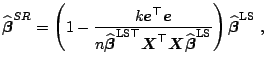
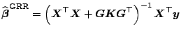
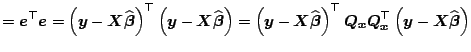
In applications, an important question remains: how to choose the
ridge parameter ![]() ?
In the original paper by [43], the use of the ridge trace,
a plot of the components of the estimated
?
In the original paper by [43], the use of the ridge trace,
a plot of the components of the estimated
![]() against
against ![]() , was
advocated. If data exhibit multicollinearity, one usually observes
a region of instability for
, was
advocated. If data exhibit multicollinearity, one usually observes
a region of instability for ![]() close to zero and then stable
estimates for large values of ridge parameter
close to zero and then stable
estimates for large values of ridge parameter ![]() . One should choose
the smallest
. One should choose
the smallest ![]() lying in the region of stable
estimates. Alternatively, one could search for
lying in the region of stable
estimates. Alternatively, one could search for ![]() minimizing
minimizing
![]() ; see the subsection on generalized
; see the subsection on generalized
![]() for more details.
Furthermore, many other methods for model selection could be employed
too; for example, LOU
for more details.
Furthermore, many other methods for model selection could be employed
too; for example, LOU
![]() (Sect. 8.1.3) performed on a grid
of
(Sect. 8.1.3) performed on a grid
of ![]() values is often used in this context.
values is often used in this context.
Statistics important for inference based on
![]() estimates are discussed
in [43] and [96] both for the case of a fixed
estimates are discussed
in [43] and [96] both for the case of a fixed ![]() as
well as in the case of some data-driven choices. Moreover, the latter
work also describes algorithms for a fast and efficient
as
well as in the case of some data-driven choices. Moreover, the latter
work also describes algorithms for a fast and efficient
![]() computation.
computation.
To conclude, let us note that the
![]() estimator
estimator
![]() in model
(8.1) can be also defined as a solution of a restricted
minimization problem
in model
(8.1) can be also defined as a solution of a restricted
minimization problem
The
![]() estimator can be generalized in the sense that each diagonal
element of
estimator can be generalized in the sense that each diagonal
element of
![]() is modified separately. To achieve that let
us recall that this matrix can be diagonalized:
is modified separately. To achieve that let
us recall that this matrix can be diagonalized:
![]() , where
, where
![]() is an
orthonormal matrix and
is an
orthonormal matrix and
![]() is a diagonal matrix containing
eigenvalues
is a diagonal matrix containing
eigenvalues
![]() .
.
The main advantage of this generalization being ridge coefficients
specific to each variable, it is important to know how to choose the
matrix
![]() . In [43]
the following result is derived.
. In [43]
the following result is derived.
An operational version (feasible
![]() ) is based on an unbiased estimate
) is based on an unbiased estimate
![]() and
and
![]() . See [43] and [96], where you
also find the bias and
. See [43] and [96], where you
also find the bias and
![]() of this operational
of this operational
![]() estimator, and
[98] for further extensions of this approach. Let us note
that the feasible
estimator, and
[98] for further extensions of this approach. Let us note
that the feasible
![]() (
(
![]() ) estimator does not have to possess the
) estimator does not have to possess the
![]() -optimality property of
-optimality property of
![]() because the optimal choice of
because the optimal choice of
![]() is replaced by an estimate. Nevertheless, the optimality property of
is replaced by an estimate. Nevertheless, the optimality property of
![]() is preserved if
is preserved if
![]() , where
, where
![]() is the
is the ![]() th-element of
th-element of
![]() ([30]).
([30]).
Additionally, given an estimate of
![]() -minimizing
-minimizing
![]() , many authors
proposed to choose the ridge parameter
, many authors
proposed to choose the ridge parameter ![]() in ordinary
in ordinary
![]() as
a harmonic mean of
as
a harmonic mean of
![]() ;
see [44], for instance.
;
see [44], for instance.
Motivated by results on
![]() , [53] proposed to correct
, [53] proposed to correct
![]() for its bias using the first-order bias approximation. This yields
almost unbiased
for its bias using the first-order bias approximation. This yields
almost unbiased
![]() (
(
![]() ) estimator
) estimator
 |
![]() can be applied also under exact multicollinearity, which arises for
example in data with more variables than observations. Although the
theory and application of
can be applied also under exact multicollinearity, which arises for
example in data with more variables than observations. Although the
theory and application of
![]() is the same as in the case of full-rank
data, the computational burden of
is the same as in the case of full-rank
data, the computational burden of
![]() operations becomes
too high for
operations becomes
too high for ![]() . A faster algorithm with computational complexity
only
. A faster algorithm with computational complexity
only ![]() was found by [39].
was found by [39].
Moreover, there are many further extensions of the
![]() principle that
go beyond the extent of this chapter. To mention at least some of
them, let us refer a reader to works comparing or combining various
ridge and shrinkage approaches [55]; [84]; [87] and to
monograph by [35].
principle that
go beyond the extent of this chapter. To mention at least some of
them, let us refer a reader to works comparing or combining various
ridge and shrinkage approaches [55]; [84]; [87] and to
monograph by [35].
![\includegraphics[width=7.5cm]{text/3-8/ridge.eps}](img5219.gif)
|
![]() discussed in Sect. 8.1.6 is very closely connected with
the continuum regression proposed by [16] as
a unifying approach to the
discussed in Sect. 8.1.6 is very closely connected with
the continuum regression proposed by [16] as
a unifying approach to the
![]() ,
,
![]() , and partial least squares (see
Sect. 8.1.9) estimation.
, and partial least squares (see
Sect. 8.1.9) estimation.
This definition yields estimates proportional to LS for
![]() ,
to
,
to
![]() for
for
![]() , and to yet-to-be-discussed partial
least squares for
, and to yet-to-be-discussed partial
least squares for
![]() . Apart from this, the advantage of
. Apart from this, the advantage of
![]() is that one can adaptively select among the methods by searching an
optimal
is that one can adaptively select among the methods by searching an
optimal ![]() . To determine
. To determine ![]() , [16] used
, [16] used
![]() .
.
The relationship between
![]() and
and
![]() was indicated already in
[90], but the most important result came after uncovering
possible discontinuities of
was indicated already in
[90], but the most important result came after uncovering
possible discontinuities of
![]() estimates as a function of data and
estimates as a function of data and
![]() by [14]. In an attempt to remedy the
discontinuity of the original
by [14]. In an attempt to remedy the
discontinuity of the original
![]() , [15] not only proposed to
maximize
, [15] not only proposed to
maximize
Thus, the
![]() estimator fundamentally underlies many methods dealing
with multicollinear and reduced rank data such as mentioned
estimator fundamentally underlies many methods dealing
with multicollinear and reduced rank data such as mentioned
![]() and
partial least squares. Notice however that negative values of the
ridge coefficient
and
partial least squares. Notice however that negative values of the
ridge coefficient ![]() have to be admitted here.
have to be admitted here.
Finally, let us note that
![]() can be extended to
multiple-response-variables models ([17]).
can be extended to
multiple-response-variables models ([17]).
The ridge regression discussed in Sect. 8.1.6 motivates
another shrinkage method: Lasso (least absolute shrinkage
and selection operator) by
[93]. Formulation (8.10) states that
![]() can be
viewed as a minimization with respect to an upper bound on the
can be
viewed as a minimization with respect to an upper bound on the ![]() norm of estimate
norm of estimate
![]() . A natural extension is to consider
constraints on the
. A natural extension is to consider
constraints on the ![]() norm
norm
![]() ,
, ![]() . Specifically,
[93] studied case of
. Specifically,
[93] studied case of ![]() , that is
, that is ![]() norm.
norm.
Lasso is a shrinkage estimator that has one specific feature compared
to ordinary
![]() . Because of the geometry of
. Because of the geometry of ![]() -norm restriction,
Lasso shrinks the effect of some variables and eliminates influence of
the others, that is, sets their coefficients to zero. Thus, it
combines regression shrinkage with variable selection, and as
[93] demonstrated also by means of simulation, it
compares favorably to all-subsets regression. In this context, it is
interesting that Lasso could be formulated as a special case of least
angle regression by [27]. Finally, let us note that to achieve
the same kind of shrinking and variable-selection effects for all
variables, they should be standardized before used in Lasso; see
[68] for details.
-norm restriction,
Lasso shrinks the effect of some variables and eliminates influence of
the others, that is, sets their coefficients to zero. Thus, it
combines regression shrinkage with variable selection, and as
[93] demonstrated also by means of simulation, it
compares favorably to all-subsets regression. In this context, it is
interesting that Lasso could be formulated as a special case of least
angle regression by [27]. Finally, let us note that to achieve
the same kind of shrinking and variable-selection effects for all
variables, they should be standardized before used in Lasso; see
[68] for details.
As far as the inference for the Lasso estimator is concerned,
[57] recently studied the asymptotic distribution of
Lasso-type estimators using ![]() -norm condition
-norm condition
![]() with
with ![]() , including behavior under nearly-singular designs.
, including behavior under nearly-singular designs.
Now, it remains to find out how Lasso estimates can be
computed. Equation (8.14)
indicates that one has to solve a restricted quadratic optimization
problem. Setting
![]() and
and
![]() , the restriction
, the restriction
![]() can be
written as
can be
written as ![]() constraints:
constraints:
![]() ,
and
,
and
![]() . Thus, convergence
is assured in
. Thus, convergence
is assured in ![]() steps. Additionally, the unknown tuning parameter
steps. Additionally, the unknown tuning parameter
![]() is to be selected by means of
is to be selected by means of
![]() . Further, although
solving (8.14) is straightforward in usual regression
problems, it can become very demanding for reduced-rank data,
. Further, although
solving (8.14) is straightforward in usual regression
problems, it can become very demanding for reduced-rank data,
![]() . [72] treated lasso as a convex programming
problem, and by formulating its dual problem, developed an efficient
algorithm usable even for
. [72] treated lasso as a convex programming
problem, and by formulating its dual problem, developed an efficient
algorithm usable even for ![]() .
.
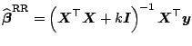
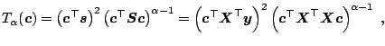
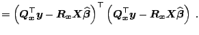
In Fig. 8.3, we can observe which variables are included in
the regression (have a nonzero coefficient) as tuning parameter ![]() increases. Clearly, the order in which the first of these variables
become significant -
increases. Clearly, the order in which the first of these variables
become significant -
![]() - closely resembles the
results of variable selection procedures in
Table 8.1. Thus, Lasso combines shrinkage estimation
and variable selection: at a given constraint level
- closely resembles the
results of variable selection procedures in
Table 8.1. Thus, Lasso combines shrinkage estimation
and variable selection: at a given constraint level ![]() , it shrinks
coefficients of some variables and removes the others by setting their
coefficients equal to zero.
, it shrinks
coefficients of some variables and removes the others by setting their
coefficients equal to zero.
![\includegraphics[width=8.6cm]{text/3-8/lasso.eps}](img5268.gif)
|
A general modeling approach to most of the methods covered so far was
![]() in Sect. 8.1.7, whereby it has two ''extremes'': LS
for
in Sect. 8.1.7, whereby it has two ''extremes'': LS
for ![]() and
and
![]() for
for
![]() . The partial
least squares (PLS) regression lies in between - it is a special
case of (8.13) for
. The partial
least squares (PLS) regression lies in between - it is a special
case of (8.13) for ![]() , see [16].
Originally proposed by [104], it was presented as an
algorithm that searches for linear combinations of explanatory
variables best explaining the dependent variable. Similarly to
, see [16].
Originally proposed by [104], it was presented as an
algorithm that searches for linear combinations of explanatory
variables best explaining the dependent variable. Similarly to
![]() ,
PLS also aims especially at situations when the number of explanatory
variables is large compared to the number of observations. Here we
present the PLS idea and algorithm themselves as well as the latest
results on variable selection and inference in PLS.
,
PLS also aims especially at situations when the number of explanatory
variables is large compared to the number of observations. Here we
present the PLS idea and algorithm themselves as well as the latest
results on variable selection and inference in PLS.
Having many explanatory variables
![]() , the aim of the PLS
method is to find a small number of linear combinations
, the aim of the PLS
method is to find a small number of linear combinations
![]() of these variables, thought about as
latent variables,
explaining observed responses
of these variables, thought about as
latent variables,
explaining observed responses
Let us now present the PLS algorithm itself, which defines yet another
shrinkage estimator as shown by [20] and [51].
(See [75] for more details and [33] for
an alternative formulation.) The indices
![]() are
constructed one after another. Estimating the intercept by
are
constructed one after another. Estimating the intercept by
![]() , let us start with centered variables
, let us start with centered variables
![]() and
and
![]() and set
and set ![]() .
.
 |
 |
This algorithm provides us with indices
![]() , which define the
analogs of principle components in
, which define the
analogs of principle components in
![]() , and the corresponding
regression coefficients
, and the corresponding
regression coefficients ![]() in (8.15). The main open
question is how to choose the number of components
in (8.15). The main open
question is how to choose the number of components ![]() . The original
method proposed by [105] is based on cross
validation. Provided that
. The original
method proposed by [105] is based on cross
validation. Provided that
![]() from (8.7)
represents the
from (8.7)
represents the
![]() index of
index of
![]() estimate with
estimate with ![]() factors, an
additional index
factors, an
additional index
![]() is added if Wold's
is added if Wold's ![]() criterion
criterion
![]() is smaller than
is smaller than ![]() .
This selects the first local minimum of the
.
This selects the first local minimum of the
![]() index, which is
superior to finding the global minimum of
index, which is
superior to finding the global minimum of
![]() as shown in
[73]. Alternatively, one can stop already when Wold's
as shown in
[73]. Alternatively, one can stop already when Wold's ![]() exceeds
exceeds ![]() or
or ![]() bound (modified Wold's
bound (modified Wold's ![]() criteria)
or to use other variable selection criteria such as
criteria)
or to use other variable selection criteria such as
![]() . In a recent
simulation study, [61] showed that modified Wold's
. In a recent
simulation study, [61] showed that modified Wold's ![]() is preferable to Wold's
is preferable to Wold's
![]() and
and
![]() . Furthermore, similarly to
. Furthermore, similarly to
![]() , there are attempts to use
, there are attempts to use
![]() for the component selection, see [58] for instance.
for the component selection, see [58] for instance.
Next, the first results on the asymptotic behavior of PLS appeared
only during last decade. The asymptotic behavior of prediction errors
was examined by [41]. The covariance matrix,
confidence and prediction intervals based on PLS estimates were first
studied by [23], but a more compact expression was
presented in [74]. It is omitted here due to many
technicalities required for its presentation. There are also attempts
to find a sample-specific prediction error of
![]() , which were compared
by [29].
, which were compared
by [29].
Finally, note that there are many extensions of the presented
algorithm, which
is usually denoted
![]() . First of all, there are extensions (
. First of all, there are extensions (
![]() ,
,
![]() , etc.) of
, etc.) of
![]() to models with multiple dependent variables, see
[50] and [32] for instance, which choose linear
combinations (latent variables) not only within explanatory variables,
but does the same also in the space spanned by dependent
variables. A recent survey of these and other so-called two-block
methods is given in [101].
to models with multiple dependent variables, see
[50] and [32] for instance, which choose linear
combinations (latent variables) not only within explanatory variables,
but does the same also in the space spanned by dependent
variables. A recent survey of these and other so-called two-block
methods is given in [101].
![]() was also adapted for
on-line process modeling, see [78] for a recursive
was also adapted for
on-line process modeling, see [78] for a recursive
![]() algorithm. Additionally, in an attempt to simplify the
interpretation of
algorithm. Additionally, in an attempt to simplify the
interpretation of
![]() results, [94] proposed orthogonalized
results, [94] proposed orthogonalized
![]() . See [108] for further details on recent
developments.
. See [108] for further details on recent
developments.
![\includegraphics[width=8.6cm]{text/3-8/pls2.eps}](img5295.gif)
|
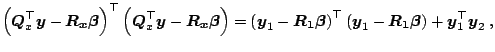
Methods discussed in Sects. 8.1.3-8.1.9 are aiming at the estimation of (nearly) singular problems and they are often very closely related, see Sect. 8.1.7. Here we provide several references to studies comparing the discussed methods.
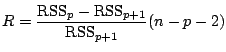
First, an extensive simulation study comparing variable selection,
![]() ,
,
![]() , and
, and
![]() regression methods is presented in
[32]. Although the results are conditional on the
simulation design used in the study, they indicate that
regression methods is presented in
[32]. Although the results are conditional on the
simulation design used in the study, they indicate that
![]() ,
,
![]() , and
, and
![]() are, in the case of ill-conditioned problems, highly preferable to
variable selection. The differences between the best methods,
are, in the case of ill-conditioned problems, highly preferable to
variable selection. The differences between the best methods,
![]() and
and
![]() , are rather small and the same holds for comparison of
, are rather small and the same holds for comparison of
![]() and
and
![]() , which seems to be slightly worse than
, which seems to be slightly worse than
![]() . An empirical
comparison of
. An empirical
comparison of
![]() and
and
![]() was also done by [103] with the
same result. Next, the fact that neither
was also done by [103] with the
same result. Next, the fact that neither
![]() , nor
, nor
![]() asymptotically
dominates the other method was proved in [41] and
further discussed in [40]. A similar asymptotic result
was also given by [88]. Finally, the fact that
asymptotically
dominates the other method was proved in [41] and
further discussed in [40]. A similar asymptotic result
was also given by [88]. Finally, the fact that
![]() should
not perform worse than
should
not perform worse than
![]() and
and
![]() is supported by
Theorem 4 in Sect. 8.1.7.
is supported by
Theorem 4 in Sect. 8.1.7.
![\includegraphics[width=7.3cm]{text/3-8/pcrplot.eps}](img5167.gif)