Survival analysis is now a standard statistical method for
lifetime data. Fundamental and classical parametric
distributions are also very important, but regression methods
are very powerful to analyze the effects of some
covariates on life lengths. [6]
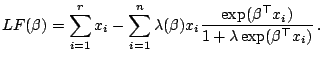
introduced a model for the hazard function
![]() with survival time
with survival time ![]() for an individual with
possibly time-dependent covariate
for an individual with
possibly time-dependent covariate ![]() , i.e.,
, i.e.,
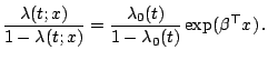
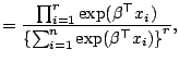
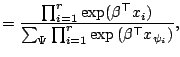
In many applications it is necessary to test the significance
of the estimated value, using for example the score test or
the likelihood ratio test based on asymptotic results of large
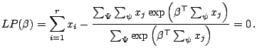
sample theory. First we express the three likelihood factors
defined at each failure time as ![]() ,
, ![]() ,
, ![]() corresponding to the Breslow-Peto,
the partial likelihood and the
generalized maximum likelihood methods, respectively;
corresponding to the Breslow-Peto,
the partial likelihood and the
generalized maximum likelihood methods, respectively;
 |
(12.19) | |
 |
(12.20) | |
 |
(12.21) |
 |
The Hessian matrices of the log likelihoods evaluated at
![]() are respectively,
are respectively,
 |
||
 |
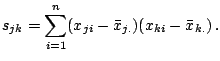 |
 |
[12] pointed out in their simulation study that
when the discrete logistic model is true the Breslow-Peto
method causes downward bias
compared to the partial likelihood method. This was proven in
[17] for any sample when ![]() is
scalar-valued, i.e.,
is
scalar-valued, i.e.,
This theorem and corollary confirm the conservatism of the Breslow-Peto approximation in relation to Cox's discrete model ([27]).
[31] proposed an approximation method using full
likelihood for the case of Cox's discrete
model. Analytically the same problems
appear in various fields of statistics. [30] and
[11] remarked that the inference procedure using the
logistic model contains the same problems in case-control studies
where data are summarized in multiple ![]() or
or ![]() tables. The proportional hazards model provides a type of logistic model for the contingency table
with ordered categories ([29]). As an extension of the
proportional hazards model, the proportional intensity model in the
point process is employed to describe an asthma attack in relation to
environmental factors ([19,31]). For convenience,
although in some cases partial likelihood becomes conditional
likelihood, we will use the term of
partial likelihood.
tables. The proportional hazards model provides a type of logistic model for the contingency table
with ordered categories ([29]). As an extension of the
proportional hazards model, the proportional intensity model in the
point process is employed to describe an asthma attack in relation to
environmental factors ([19,31]). For convenience,
although in some cases partial likelihood becomes conditional
likelihood, we will use the term of
partial likelihood.
It is worthwhile to explore the behavior of the maximum full likelihood estimator even when the maximum partial likelihood estimator is applicable. Both estimators obviously behave similarly in a rough sense, yet they are different in details. Identifying differences between the two estimators should be helpful in choosing one of the two.
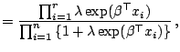
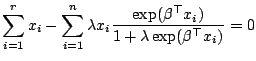
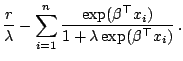
We use the notation described in the previous section for expressing the two likelihoods. Differentiating
![]() gives
gives
 |
Differentiating
![]() with respect to
with respect to ![]() and
and
![]() allows obtaining the maximum full likelihood
estimator, i.e.,
allows obtaining the maximum full likelihood
estimator, i.e.,
 |
 |
 |
Note that the entire likelihoods are the products over all
distinct failure times ![]() . Thus the likelihood equations in
a strict sense are
. Thus the likelihood equations in
a strict sense are
![]() and
and
![]() , where the summations extend over
, where the summations extend over ![]() in
in ![]() .
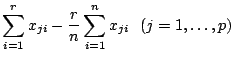
As far as we are concerned, the results in a single failure
time can be straightforwardly extended to those with multiple
failure times. Let us now focus on likelihood equations of
a single failure time and suppress the suffix
.
As far as we are concerned, the results in a single failure
time can be straightforwardly extended to those with multiple
failure times. Let us now focus on likelihood equations of
a single failure time and suppress the suffix ![]() .
.
Extension to the case of vector parameter ![]() is
straightforward. From Proposition 1 it follows that if either
of the two estimators exists, then the other also exists and
they are uniquely determined. Furthermore, both the estimators
have a common sign.
is
straightforward. From Proposition 1 it follows that if either
of the two estimators exists, then the other also exists and
they are uniquely determined. Furthermore, both the estimators
have a common sign.
To quantitatively compare the behaviors of ![]() and
and
![]() , their their power expansions are presented near the origin. Since both
functions behave similarly, it is expected that the
quantitative difference near the origin is critical over
a wide range of
, their their power expansions are presented near the origin. Since both
functions behave similarly, it is expected that the
quantitative difference near the origin is critical over
a wide range of ![]() . Behavior near the origin is of
practical importance for studying the estimator and test
procedure.
. Behavior near the origin is of
practical importance for studying the estimator and test
procedure.
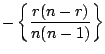
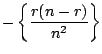
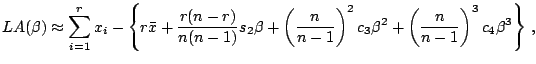
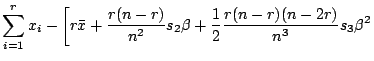 |
||
![$\displaystyle +\left.\frac{1}{6}\frac{r(n-r)}{n^5}\left\{n(n^2-6rn+6r^2)s_4 - 3(n-2r)^2s_2^2\right\}\beta^3\right],$](img6606.gif) |
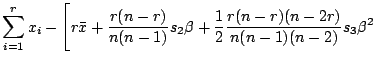 |
||
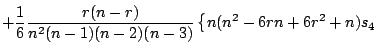 |
||
![$\displaystyle \left.+ 3(r-1)n(n-r-1)s_2^2\right\}\beta^3\Biggr]\,,$](img6610.gif) |
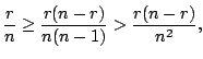
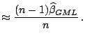
The function ![]() has a steeper slope near the origin
than
has a steeper slope near the origin
than ![]() . The relative ratio is
. The relative ratio is ![]() , which
indicates that
, which
indicates that
![]() is close to
is close to ![]() near
the origin. The power expansion of
near
the origin. The power expansion of
![]() is expressed by
is expressed by
 |
(12.23) |
| (12.24) | ||
 |
(12.25) |
The proposed approximated estimator and test statistic are
quite helpful in cases of multiple ![]() table when the value of both
table when the value of both ![]() and
and
![]() are large ([31]).
are large ([31]).