Boosting algorithms have been prpoposed in the machine learning
literature by Schapire ([47]) and Freund
([30], [31]), see also ([48]). These first
algorithms have been developed as ensemble methods. Unlike bagging
which is a parallel ensemble method, boosting methods are
sequential ensemble algorithms where the weights ![]() in
(16.1) are depending on the previous fitted functions
in
(16.1) are depending on the previous fitted functions
![]() . Boosting has been empirically
demonstrated to be very accurate in terms of classification,
notably the so-called AdaBoost algorithm ([31]).
. Boosting has been empirically
demonstrated to be very accurate in terms of classification,
notably the so-called AdaBoost algorithm ([31]).
We will explain below that boosting can be viewed as a nonparametric optimization algorithm in function space, as first pointed out by Breiman ([11], [12]). This view turns out to be very fruitful to adapt boosting for other problems than classification, including regression and survival analysis.
Maybe it is worth mentioning here that boosting algorithms have often better predictive power than bagging, (cf. ([11])); of course, such a statement has to be read with caution, and methods should be tried out on individual data-sets, including e.g. cross-validation, before selecting one among a few methods.
To give an idea, we report here some empirical results from ([11]) for classification: we show below the gains (in percentage) of boosting trees over bagging trees:
| ''normal'' size data-sets: | ||||
| large data-sets: |
Rather than looking through the lenses of ensemble methods, boosting
algorithms can be seen as functional gradient descent techniques
([11], [12]). The goal is to estimate a function
![]() , minimizing an expected loss
, minimizing an expected loss
As we will see in Sect. 16.3.2, boosting algorithms are pursuing a ''small'' empirical risk
 |
The most popular loss functions, for regression and binary classification, are given in Table 16.1.
| Boosting | Loss function | Population minimizer for (16.11) |
|
|
|
|
| LogitBoost |
|
|
| AdaBoost |
|
|
While the squared error loss is mainly used for regression (see ([19]) for classification with the squared error loss), the log-likelihood and the exponential loss are for binary classification only.
The form of the log-likelihood loss may be somewhat unusual: we norm
it, by using the base ![]() so that it ''touches'' the
misclassification error as an upper bound (see Fig. 16.3),
and we write it as a function of the so-called margin
so that it ''touches'' the
misclassification error as an upper bound (see Fig. 16.3),
and we write it as a function of the so-called margin
![]() , where
, where
![]() is the usual
labeling from the machine learning community. Thus, the loss is
a function of the margin
is the usual
labeling from the machine learning community. Thus, the loss is
a function of the margin
![]() only; and the same is true with
the exponential loss and also the squared error loss for
classification since
only; and the same is true with
the exponential loss and also the squared error loss for
classification since
![\includegraphics[height=6.3333cm,width=9cm,clip]{text/3-16/abb/loss.eps}](img7227.gif)
|
The misclassification loss, or zero-one loss, is
![]() , again a function of the margin, whose population minimizer is
, again a function of the margin, whose population minimizer is
![]() . For readers less
familiar with the concept of the margin, this can also be understood
as follows: the Bayes-classifier which minimizes the misclassification
risk is
. For readers less
familiar with the concept of the margin, this can also be understood
as follows: the Bayes-classifier which minimizes the misclassification
risk is
The (surrogate) loss functions given in Table 16.1 are all
convex functions of the margin
![]() which bound the zero-one
misclassification loss from above, see Fig. 16.3. The
convexity of these surrogate loss functions is computationally
important for empirical risk minimization; minimizing the empirical
zero-one loss is computationally intractable.
which bound the zero-one
misclassification loss from above, see Fig. 16.3. The
convexity of these surrogate loss functions is computationally
important for empirical risk minimization; minimizing the empirical
zero-one loss is computationally intractable.
Estimation of the function ![]() , which minimizes an expected
loss in (16.11), is pursued by a constrained
minimization of the empirical risk
, which minimizes an expected
loss in (16.11), is pursued by a constrained
minimization of the empirical risk
![]() . The constraint comes in algorithmically (and
not explicitly), by the way we are attempting to minimize the
empirical risk, with a so-called functional gradient descent. This
gradient descent view has been recognized and refined by various
authors (cf. ([11], [12], [43], [34],
[33], [19])). In summary, the minimizer of the
empirical risk is imposed to satisfy a ''smoothness'' constraint
in terms of a linear expansion of (''simple'') fits from
a real-valued base procedure function estimate.
. The constraint comes in algorithmically (and
not explicitly), by the way we are attempting to minimize the
empirical risk, with a so-called functional gradient descent. This
gradient descent view has been recognized and refined by various
authors (cf. ([11], [12], [43], [34],
[33], [19])). In summary, the minimizer of the
empirical risk is imposed to satisfy a ''smoothness'' constraint
in terms of a linear expansion of (''simple'') fits from
a real-valued base procedure function estimate.
Step 1 (initialization). Given data
![]() , apply the base procedure yielding the function estimate
, apply the base procedure yielding the function estimate
Step 2 (projecting gradient to learner). Compute the
negative gradient vector
 |
Step 3 (line search). Do a one-dimensional numerical search for the
best step-size
 |
Step 4 (iteration). Increase ![]() by one and repeat
Steps 2 and 3 until a stopping iteration
by one and repeat
Steps 2 and 3 until a stopping iteration ![]() is achieved.
is achieved.
The number of iterations ![]() is the tuning parameter of boosting. The
larger it is, the more complex the estimator. But the complexity, for
example the variance of the estimator, is not linearly increasing in
is the tuning parameter of boosting. The
larger it is, the more complex the estimator. But the complexity, for
example the variance of the estimator, is not linearly increasing in
![]() : instead, it increases very slowly as
: instead, it increases very slowly as ![]() gets larger, see also
Fig. 16.4 in Sect. 16.3.5.
gets larger, see also
Fig. 16.4 in Sect. 16.3.5.
Obviously, the choice of the base procedure influences the boosting
estimate. Originally, boosting has been mainly used with tree-type
base procedures, typically with small trees such as stumps (two
terminal nodes) or trees having say ![]() terminal nodes
(cf. ([11], [14], [7], [34],
[25])); see also
Sect. 16.3.8. But we will demonstrate in
Sect. 16.3.6 that boosting may be very worthwhile within
the class of linear, additive or interaction models, allowing for good
model interpretation.
terminal nodes
(cf. ([11], [14], [7], [34],
[25])); see also
Sect. 16.3.8. But we will demonstrate in
Sect. 16.3.6 that boosting may be very worthwhile within
the class of linear, additive or interaction models, allowing for good
model interpretation.
The function estimate
![]() in Step 2 can be viewed as an
estimate of
in Step 2 can be viewed as an
estimate of
![]() , the expected negative gradient given the
predictor
, the expected negative gradient given the
predictor ![]() , and takes values in
, and takes values in
![]() , even in case of
a classification problem with
, even in case of
a classification problem with ![]() in a finite set (this is different
from the AdaBoost algorithm, see below).
in a finite set (this is different
from the AdaBoost algorithm, see below).
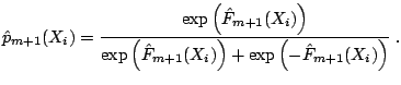
We call
![]() the
the ![]() Boost-, LogitBoost- or
AdaBoost-estimate, according to the implementing loss function
Boost-, LogitBoost- or
AdaBoost-estimate, according to the implementing loss function
![]() ,
,
![]() or
or
![]() ,
respectively; see Table 16.1.
,
respectively; see Table 16.1.
The original AdaBoost algorithm for classification is actually a bit
different: the base procedure fit is a classifier, and not
a real-valued estimator for the conditional probability of ![]() given
given
![]() ; and Steps 2 and 3 are also somewhat different. Since AdaBoost's
implementing exponential loss function is not well established in
statistics, we refer for a detailed discussion to ([34]). From
a statistical perspective, the squared error loss and log-likelihood
loss functions are most prominent and we describe below the
corresponding boosting algorithms in detail.
; and Steps 2 and 3 are also somewhat different. Since AdaBoost's
implementing exponential loss function is not well established in
statistics, we refer for a detailed discussion to ([34]). From
a statistical perspective, the squared error loss and log-likelihood
loss functions are most prominent and we describe below the
corresponding boosting algorithms in detail.
Boosting using the squared error loss, ![]() Boost, has a simple
structure: the negative gradient in Step 2 is the classical residual
vector and the line search in Step 3 is trivial when using a base
procedure which does least squares fitting.
Boost, has a simple
structure: the negative gradient in Step 2 is the classical residual
vector and the line search in Step 3 is trivial when using a base
procedure which does least squares fitting.
Step 1 (initialization). As in Step 1 of generic functional gradient descent.
Step 2. Compute residuals
![]() and fit the real-valued base procedure to the current residuals
(typically by (penalized) least squares) as in Step 2 of the generic
functional gradient descent; the fit is
denoted by
and fit the real-valued base procedure to the current residuals
(typically by (penalized) least squares) as in Step 2 of the generic
functional gradient descent; the fit is
denoted by
![]() .
.
Update
Step 3 (iteration). Increase iteration
index ![]() by one and repeat Step 2 until a stopping iteration
by one and repeat Step 2 until a stopping iteration ![]() is
achieved.
is
achieved.
The estimate
![]() is an estimator of the
regression function
is an estimator of the
regression function
![]() .
. ![]() Boosting is nothing else
than repeated least squares fitting of residuals
(cf. ([33], [19])). With
Boosting is nothing else
than repeated least squares fitting of residuals
(cf. ([33], [19])). With ![]() (one boosting step), it has
already been proposed by Tukey ([51]) under the name
''twicing''. In the non-stochastic context, the
(one boosting step), it has
already been proposed by Tukey ([51]) under the name
''twicing''. In the non-stochastic context, the ![]() Boosting
algorithm is known as ''Matching Pursuit'' ([41]) which is
popular in signal processing for fitting overcomplete dictionaries.
Boosting
algorithm is known as ''Matching Pursuit'' ([41]) which is
popular in signal processing for fitting overcomplete dictionaries.
Boosting using the log-likelihood loss for binary classification (and more generally for multi-class problems) is known as LogitBoost ([34]). LogitBoost uses some Newton-stepping with the Hessian, rather than the line search in Step 3 of the generic boosting algorithm:
Step 1 (initialization). Start with
conditional probability estimates
![]() (for
(for
![]() ). Set
). Set ![]() .
.
Step 2. Compute the pseudo-response
(negative gradient)
 |
 |
Step 3 (iteration). Increase iteration
index ![]() by one and repeat Step 2 until a stopping iteration
by one and repeat Step 2 until a stopping iteration ![]() is
achieved.
is
achieved.
The estimate
![]() is an estimator for half of
the log-odds ratio
is an estimator for half of
the log-odds ratio
![]() logit
logit![]() (see
Table 16.1). Thus, a classifier (under equal misclassification
loss for the labels
(see
Table 16.1). Thus, a classifier (under equal misclassification
loss for the labels ![]() and
and ![]() ) is
) is
| sign |
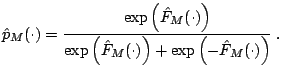 |
The LogitBoost algorithm described above can be modified for
multi-class problems where the response variable takes values in
a finite set
![]() with
with ![]() by using the
multinomial log-likelihood loss ([34]). But sometimes it can be
advantageous to run instead a binary classifier (e.g. with boosting)
for many binary problems. The most common approach is to code for
by using the
multinomial log-likelihood loss ([34]). But sometimes it can be
advantageous to run instead a binary classifier (e.g. with boosting)
for many binary problems. The most common approach is to code for ![]() binary problems where the
binary problems where the ![]() th problem assigns the response
th problem assigns the response
![$\displaystyle Y^{(j)} = \begin{cases}1\;, & \text{if}\;\; Y=j\;,\\ [1.5mm] 0\;, & \text{if}\;\; Y \neq j\;. \end{cases}$](img7270.gif) |
Other codings of a multi-class into into multiple binary problems are discussed in ([1]).
It is often better to use small step sizes instead of using the full
line search step-length
![]() from Step 3 in the generic
boosting algorithm (or
from Step 3 in the generic
boosting algorithm (or
![]() for
for ![]() Boost or
Boost or
![]() for LogitBoost). We advocate here to use
the step-size
for LogitBoost). We advocate here to use
the step-size
We discuss here the behavior of boosting in terms of model-complexity
and estimation error when the number of iterations increase. This is
best understood in the framework of squared error loss and
![]() Boosting.
Boosting.
We represent the base procedure as an operator
 |
The case where the base procedure is a smoothing spline for
a one-dimensional predictor
![]() is instructive, although
being only a toy example within the range of potential applications of
boosting algorithms.
is instructive, although
being only a toy example within the range of potential applications of
boosting algorithms.
In our notation from above,
![]() denotes a smoothing spline operator
which is the solution (
denotes a smoothing spline operator
which is the solution (
![]() ) of the
following optimization problem (cf. ([54]))
) of the
following optimization problem (cf. ([54]))
 |
Within the class of smoothing spline base procedures, we choose
a spline by fixing a smoothing parameter ![]() . This should be
done such that the base procedure has low variance but potentially
high bias: for example, we may choose
. This should be
done such that the base procedure has low variance but potentially
high bias: for example, we may choose ![]() such that the degrees
of freedom
such that the degrees
of freedom
![]() trace
trace![]() is low, e.g.
is low, e.g. ![]() . Although
the base procedure has typically high bias, we will reduce it by
pursuing suitably many boosting iterations. Choosing the
. Although
the base procedure has typically high bias, we will reduce it by
pursuing suitably many boosting iterations. Choosing the ![]() is not
really a tuning parameter: we only have to make sure that
is not
really a tuning parameter: we only have to make sure that ![]() is
small enough, so that the initial estimate (or first few boosting
estimates) are not already overfitting. This is easy to achieve in
practice and a theoretical characterization is described
in ([19]).
is
small enough, so that the initial estimate (or first few boosting
estimates) are not already overfitting. This is easy to achieve in
practice and a theoretical characterization is described
in ([19]).
Related aspects of choosing the base procedure are described in Sects. 16.3.6 and 16.3.8. The general ''principle'' is to choose a base procedure which has low variance and having the property that when taking linear combinations thereof, we obtain a model-class which is rich enough for the application at hand.
As boosting iterations proceed, the bias of the estimator will go down
and the variance will increase. However, this bias-variance exhibits
a very different behavior as when classically varying the smoothing
parameter (the parameter ![]() ). It can be shown that the variance
increases with exponentially small increments of the order
). It can be shown that the variance
increases with exponentially small increments of the order
![]() , while the bias decays quickly: the optimal mean
squared error for the best boosting iteration
, while the bias decays quickly: the optimal mean
squared error for the best boosting iteration ![]() is (essentially) the
same as for the optimally selected tuning parameter
is (essentially) the
same as for the optimally selected tuning parameter ![]() ([19]), but the trace of the mean squared error is very
different, see Fig. 16.4. The
([19]), but the trace of the mean squared error is very
different, see Fig. 16.4. The ![]() Boosting method is much
less sensitive to overfitting and hence often easier to tune. The
mentioned insensitivity about overfitting also applies to
higher-dimensional problems, implying potential advantages about
tuning.
Boosting method is much
less sensitive to overfitting and hence often easier to tune. The
mentioned insensitivity about overfitting also applies to
higher-dimensional problems, implying potential advantages about
tuning.
![\includegraphics[height=5.928cm,width=8.3cm]{text/3-16/abb/pbyu.newadd3.eps}](img7296.gif)
|
Such ![]() Boosting with smoothing splines achieves the asymptotically
optimal minimax MSE rates, and the method can even adapt to higher
order smoothness of the true underlying function, without knowledge of
the true degree of smoothness ([19]).
Boosting with smoothing splines achieves the asymptotically
optimal minimax MSE rates, and the method can even adapt to higher
order smoothness of the true underlying function, without knowledge of
the true degree of smoothness ([19]).
In Sect. 16.3.4, we already pointed out that
![]() Boosting yields another way of regularization by seeking for
a compromise between bias and variance. This regularization turns out
to be particularly powerful in the context with many predictor
variables.
Boosting yields another way of regularization by seeking for
a compromise between bias and variance. This regularization turns out
to be particularly powerful in the context with many predictor
variables.
Consider the component-wise smoothing spline which is defined as
a smoothing spline with one selected predictor variable
![]() (
(
![]() ), where
), where
 |
![]() Boost with component-wise smoothing splines yields an additive
model, since in every boosting iteration, a function of one selected
predictor variable is linearly added to the current fit and hence, we
can always rearrange the summands to represent the boosting estimator
as an additive function in the original variables,
Boost with component-wise smoothing splines yields an additive
model, since in every boosting iteration, a function of one selected
predictor variable is linearly added to the current fit and hence, we
can always rearrange the summands to represent the boosting estimator
as an additive function in the original variables,
![]() . The estimated functions
. The estimated functions
![]() are fitted in a stage-wise fashion and they are
different from the backfitting estimates in additive models
(cf. ([35])). Boosting has much greater flexibility to add
complexity, in a stage-wise fashion: in particular, boosting does
variable selection, since some of the predictors will never be chosen,
and it assigns variable amount of degrees of freedom to the selected
components (or function estimates); the degrees of freedom are defined
below. An illustration of this interesting way to fit additive
regression models with high-dimensional predictors is given in
Figs. 16.5 and 16.6 (actually, a penalized version of
are fitted in a stage-wise fashion and they are
different from the backfitting estimates in additive models
(cf. ([35])). Boosting has much greater flexibility to add
complexity, in a stage-wise fashion: in particular, boosting does
variable selection, since some of the predictors will never be chosen,
and it assigns variable amount of degrees of freedom to the selected
components (or function estimates); the degrees of freedom are defined
below. An illustration of this interesting way to fit additive
regression models with high-dimensional predictors is given in
Figs. 16.5 and 16.6 (actually, a penalized version of
![]() Boosting, as described below, is shown).
Boosting, as described below, is shown).
When using regression stumps (decision trees having two terminal
nodes) as the base procedure, we also get an additive model fit (by
the same argument as with component-wise smoothing splines). If the
additive terms
![]() are smooth functions of the predictor
variables, the component-wise smoothing spline is often a better base
procedure than stumps ([19]). For the purpose of
classification, e.g. with LogitBoost, stumps often seem to do a decent
job; also, if the predictor variables are non-continuous,
component-wise smoothing splines are often inadequate.
are smooth functions of the predictor
variables, the component-wise smoothing spline is often a better base
procedure than stumps ([19]). For the purpose of
classification, e.g. with LogitBoost, stumps often seem to do a decent
job; also, if the predictor variables are non-continuous,
component-wise smoothing splines are often inadequate.
Finally, if the number ![]() of predictors is ''reasonable'' in
relation to sample size
of predictors is ''reasonable'' in
relation to sample size ![]() , boosting techniques are not necessarily
better than more classical estimation methods ([19]). It seems
that boosting has most potential when the predictor dimension is very
high ([19]). Presumably, more classical methods become then
very difficult to tune while boosting seems to produce a set of
solutions (for every boosting iteration another solution) whose best
member, chosen e.g. via cross-validation, has often very good
predictive performance. A reason for the efficiency of the trace of
boosting solutions is given in Sect. 16.3.9.
, boosting techniques are not necessarily
better than more classical estimation methods ([19]). It seems
that boosting has most potential when the predictor dimension is very
high ([19]). Presumably, more classical methods become then
very difficult to tune while boosting seems to produce a set of
solutions (for every boosting iteration another solution) whose best
member, chosen e.g. via cross-validation, has often very good
predictive performance. A reason for the efficiency of the trace of
boosting solutions is given in Sect. 16.3.9.
For component-wise base procedures, which pick one or also a pair of
variables at the time, all the component-wise fitting operators are
involved: for simplicity, we focus on additive modeling with
component-wise fitting operators
![]() , e.g. the
component-wise smoothing spline.
, e.g. the
component-wise smoothing spline.
The boosting operator, when using the step size
![]() , is
then of the form
, is
then of the form
If the
![]() 's are all linear operators, and ignoring the effect of
selecting the components, it is reasonable to define the degrees of
boosting as
's are all linear operators, and ignoring the effect of
selecting the components, it is reasonable to define the degrees of
boosting as
We can represent
 |
 |
|
Having some degrees of freedom at hand, we can now use the AIC, or
some corrected version thereof, to define a stopping rule of boosting
without doing some sort of cross-validation: the corrected AIC
statistic ([38]) for boosting in the ![]() th iteration is
th iteration is
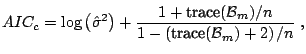 |
(16.12) |
 |
(16.13) |
Alternatively, we could use generalized cross-validation
(cf. ([36])), which involves degrees of freedom. This would
exhibit the same computational advantage, as ![]() , over
cross-validation: instead of running boosting multiple times,
, over
cross-validation: instead of running boosting multiple times, ![]() and generalized cross-validation need only one run of boosting (over
a suitable number of iterations).
and generalized cross-validation need only one run of boosting (over
a suitable number of iterations).
When viewing the ![]() criterion in (16.12) as a reasonable
estimate of the true underlying mean squared error (ignoring
uninteresting constants), we may attempt to construct a boosting
algorithm which reduces in every step the
criterion in (16.12) as a reasonable
estimate of the true underlying mean squared error (ignoring
uninteresting constants), we may attempt to construct a boosting
algorithm which reduces in every step the ![]() statistic (an
estimate of the out-sample MSE) most, instead of maximally reducing
the in-sample residual sum of squares.
statistic (an
estimate of the out-sample MSE) most, instead of maximally reducing
the in-sample residual sum of squares.
We describe here penalized boosting for additive model fitting using individual smoothing splines:
Step 1 (initialization). As in Step 1 of
![]() Boost by fitting a component-wise smoothing spline.
Boost by fitting a component-wise smoothing spline.
Step 2. Compute residuals
![]() . Choose the individual smoothing
spline which reduces
. Choose the individual smoothing
spline which reduces ![]() most: denote the selected component by
most: denote the selected component by
![]() and the fitted function, using the selected
component
and the fitted function, using the selected
component
![]() by
by
![]() .
.
Update
Step 3 (iteration). Increase iteration
index ![]() by one and repeat Step 2 until the
by one and repeat Step 2 until the ![]() criterion
in (16.12) cannot be improved anymore.
criterion
in (16.12) cannot be improved anymore.
This algorithm cannot be written in terms of fitting a base
procedure multiple times since selecting the component
![]() in Step 2 not only depends on the residuals
in Step 2 not only depends on the residuals
![]() , but
also on the degrees of boosting,
i.e.
trace
, but
also on the degrees of boosting,
i.e.
trace![]() ; the latter is a complicated,
although linear function, of the boosting iterations
; the latter is a complicated,
although linear function, of the boosting iterations
![]() . Penalized
. Penalized ![]() Boost yields more sparse solutions
than the corresponding
Boost yields more sparse solutions
than the corresponding ![]() Boost (with component-wise smoothing
splines as corresponding base procedure). The reason is that
Boost (with component-wise smoothing
splines as corresponding base procedure). The reason is that
![]() increases only little in iteration
increases only little in iteration ![]() , if the
, if the ![]() th
selected predictor variables has already been selected many times in
previous iterations; this is directly connected to the slow increase
in variance and overfitting as exemplified in Fig. 16.4.
th
selected predictor variables has already been selected many times in
previous iterations; this is directly connected to the slow increase
in variance and overfitting as exemplified in Fig. 16.4.
An illustration of penalized ![]() Boosting with individual smoothing
splines is shown in Figs. 16.5 and 16.6, based on
simulated data. The simulation model is
Boosting with individual smoothing
splines is shown in Figs. 16.5 and 16.6, based on
simulated data. The simulation model is
 |
|
| (16.14) |
![\includegraphics[width=11.7cm]{text/3-16/abb/boost-dsc2003.2.eps}](img7339.gif)
|
![\includegraphics[width=11.7cm]{text/3-16/abb/boost-dsc2003.4.eps}](img7340.gif)
|
In terms of prediction performance, penalized ![]() Boosting is not
always better than
Boosting is not
always better than ![]() Boosting; Fig. 16.7 illustrates an
advantage of penalized
Boosting; Fig. 16.7 illustrates an
advantage of penalized ![]() Boosting. But penalized
Boosting. But penalized ![]() Boosting is
always sparser (or at least not less sparse) than the corresponding
Boosting is
always sparser (or at least not less sparse) than the corresponding
![]() Boosting.
Boosting.
Obviously, penalized ![]() Boosting can be used for other than additive
smoothing spline model fitting. The modifications are straightforward
as long as the individual base procedures are linear operators.
Boosting can be used for other than additive
smoothing spline model fitting. The modifications are straightforward
as long as the individual base procedures are linear operators.
![]() Boosting for additive modeling can be easily extended to
interaction modeling (having low degree of interaction). Among the
most prominent case is the second order interaction model
Boosting for additive modeling can be easily extended to
interaction modeling (having low degree of interaction). Among the
most prominent case is the second order interaction model
![]() , where
, where
![]() .
.
Boosting with a pairwise thin plate spline, which selects the best pair of predictor variables yielding lowest residual sum of squares (when having the same degrees of freedom for every thin plate spline), yields a second-order interaction model. We demonstrate in Fig. 16.7 the effectiveness of this procedure in comparison with the second-order MARS fit ([32]). The underlying model is the Friedman #1 model:
 |
|
| (16.15) |
In high-dimensional settings, it seems that such interaction
![]() Boosting is clearly better than the more classical MARS fit,
while both of them share the same superb simplicity of interpretation.
Boosting is clearly better than the more classical MARS fit,
while both of them share the same superb simplicity of interpretation.
![\includegraphics[height=10cm]{text/3-16/abb/forthfit-dsc2003.eps}](img7349.gif)
|
![]() Boosting turns out to be also very useful for linear models when
there are many predictor variables. An attractive base procedure is
component-wise linear least squares regression, using the one selected
predictor variables which reduces residual sum of squares most.
Boosting turns out to be also very useful for linear models when
there are many predictor variables. An attractive base procedure is
component-wise linear least squares regression, using the one selected
predictor variables which reduces residual sum of squares most.
This method does variable selection, since some of the predictors will
never be picked during boosting iterations; and it assigns variable
amount of degrees of freedom (or shrinkage), as discussed for additive
models above. Recent theory shows that this method is consistent for
very high-dimensional problems where the number of predictors ![]() is allowed to grow like
is allowed to grow like
![]() , but the true
underlying regression coefficients are sparse in terms of their
, but the true
underlying regression coefficients are sparse in terms of their
![]() -norm, i.e.
-norm, i.e.
![]() , where
, where ![]() is the vector of regression
coefficients ([16]).
is the vector of regression
coefficients ([16]).
The most popular base procedures for boosting, at least in the machine
learning community, are trees. This may be adequate for
classification, but when it comes to regression, or also estimation of
conditional probabilities
![]() in classification, smoother
base procedures often perform better if the underlying regression or
probability curve is a smooth function of continuous predictor
variables ([19]).
in classification, smoother
base procedures often perform better if the underlying regression or
probability curve is a smooth function of continuous predictor
variables ([19]).
Even when using trees, the question remains about the size of the
tree. A guiding principle is as follows: take the smallest trees, i.e.
trees with the smallest number ![]() of terminal nodes, such that the
class of linear combinations of
of terminal nodes, such that the
class of linear combinations of ![]() -node trees is sufficiently rich
for the phenomenon to be modeled; of course, there is also here
a trade-off between sample size and the complexity of the function
class.
-node trees is sufficiently rich
for the phenomenon to be modeled; of course, there is also here
a trade-off between sample size and the complexity of the function
class.
For example, when taking stumps with ![]() , the set of linear
combinations of stumps is dense in (or ''yields'' the) set of
additive functions ([14]). In ([34]), this is demonstrated
from a more practical point of view. When taking trees with three
terminal nodes (
, the set of linear
combinations of stumps is dense in (or ''yields'' the) set of
additive functions ([14]). In ([34]), this is demonstrated
from a more practical point of view. When taking trees with three
terminal nodes (![]() ), the set of linear combinations of 3-node trees
yields all second-order interaction functions. Thus, when aiming for
consistent estimation of the full regression (or conditional
class-probability) function, we should choose trees with
), the set of linear combinations of 3-node trees
yields all second-order interaction functions. Thus, when aiming for
consistent estimation of the full regression (or conditional
class-probability) function, we should choose trees with ![]() terminal nodes (in practice only if the sample size is
''sufficiently large'' in relation to
terminal nodes (in practice only if the sample size is
''sufficiently large'' in relation to ![]() ), (cf. ([14])).
), (cf. ([14])).
Consistency of the AdaBoost algorithm is proved in ([39]),
for example when using trees having ![]() terminal nodes. More
refined results are given in ([42], [55]) for modified
boosting procedures with more general loss functions.
terminal nodes. More
refined results are given in ([42], [55]) for modified
boosting procedures with more general loss functions.
The main disadvantage from a statistical perspective is the lack of interpretation when boosting trees. This is in sharp contrast to boosting for linear, additive or interaction modeling. An approach to enhance interpretation is described in ([33]).
Another method which does variable selection and variable amount of
shrinkage is basis pursuit ([22]) or Lasso ([50]) which
employs an ![]() -penalty for the coefficients in the
log-likelihood.
-penalty for the coefficients in the
log-likelihood.
Interestingly, in case of linear least squares regression with a
''positive cone condition'' on the design matrix, an approximate
equivalence of (a version of) ![]() Boosting and Lasso has been
demonstrated in ([29]). More precisely, the set of boosting
solutions, when using an (infinitesimally) small step size (see
Sect. 16.3.3), over all the different boosting
iterations, equals approximately the set of Lasso solutions when
varying the
Boosting and Lasso has been
demonstrated in ([29]). More precisely, the set of boosting
solutions, when using an (infinitesimally) small step size (see
Sect. 16.3.3), over all the different boosting
iterations, equals approximately the set of Lasso solutions when
varying the ![]() -penalty parameter. Moreover, the approximate set
of boosting solutions can be computed very efficiently by the
so-called least angle regression algorithm ([29]).
-penalty parameter. Moreover, the approximate set
of boosting solutions can be computed very efficiently by the
so-called least angle regression algorithm ([29]).
It is not clear to what extent this approximate equivalence between boosting and Lasso carries over to more general design matrices in linear regression or to other problems than regression with other loss functions. But the approximate equivalence in the above mentioned special case may help to understand boosting from a different perspective.
In the machine learning community, there has been a substantial focus on consistent estimation in the convex hull of function classes (cf. ([5], [6], [40])). For example, one may want to estimate a regression or probability function which can be written as
 |
Boosting, or functional gradient descent, has also been proposed for other settings than regression or classification, including survival analysis ([8]), ordinal response problems ([52]) and high-multivariate financial time series ([4], [3]).
Support vector machines (cf. ([53], [36], [49]) have become very popular in classification due to their good performance in a variety of data sets, similarly as boosting methods for classification. A connection between boosting and support vector machines has been made in ([46]), suggesting also a modification of support vector machines to more sparse solutions ([56]).
Acknowledgements. I would like to thank Marcel Dettling for some constructive comments.