Subsections

• 4.3.1 General Principle of Iterative Methods for Linear Systems
• 4.3.2 Jacobi Method
• 4.3.3 Gauss-Seidel Method
• 4.3.4 Successive Overrelaxation Method
• 4.3.5 Gradient Methods
  • 4.3.5.1 Gauss-Seidel Method as a Gradient Method
  • 4.3.5.2 Steepest Descent Method
  • 4.3.5.3 Conjugate Gradient Method

4.3 Iterative Methods
for Solving Linear Systems

Direct methods for solving linear systems theoretically give the exact solution in a finite number of steps, see Sect. 4.2. Unfortunately, this is rarely true in applications because of rounding errors: an error made in one step spreads further in all following steps! Contrary to direct methods, iterative methods construct a series of solution approximations such that it converges to the exact solution of a system. Their main advantage is that they are self-correcting, see Sect. 4.3.1.

In this section, we first discuss general principles of iterative methods that solve linear system (4.6), $\boldsymbol{A} \boldsymbol{x} = \boldsymbol{b}$, whereby we assume that $\boldsymbol{A}\in {\mathbb{R}}^{n\times n}$ and the system has exactly one solution  $\boldsymbol{x}_{e}$ (see Sect. 4.2 for more details on other cases). Later, we describe most common iterative methods: the Jacobi, Gauss-Seidel, successive overrelaxation, and gradient methods (Sects. 4.3.2-4.3.5). Monographs containing detailed discussion of these methods include [7,24] and [27]. Although we treat these methods separately from the direct methods, let us mention here that iterative methods can usually benefit from a combination with the Gauss elimination, see [46] and [1], for instance.

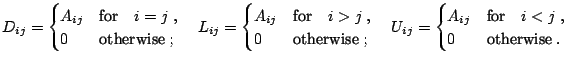
To unify the presentation of all methods, let $\boldsymbol{D}$, $\boldsymbol{L}$, and $\boldsymbol{U}$ denote the diagonal, lower triangular and upper triangular parts of a matrix $\boldsymbol{A}$ throughout this section:

$$D_{ij} = \begin{cases}A_{ij} & \text{for}\quad i=j\;,\\ 0 & \text... ...gin{cases}A_{ij} & \text{for}\quad i<j\;,\\ 0 & \text{otherwise}\;. \end{cases}$$

4.3.1 General Principle
of Iterative Methods for Linear Systems

An iterative method for solving a linear system $\boldsymbol{A} \boldsymbol{x} = \boldsymbol{b}$ constructs an iteration series $\boldsymbol{x}_i$, $i = 0,1,2,\ldots$, that under some conditions converges to the exact solution  $\boldsymbol{x}_{e}$ of the system ( $\boldsymbol{A} \boldsymbol{x}_{e} = \boldsymbol{b}$). Thus, it is necessary to choose a starting point $\boldsymbol{x}_0$ and iteratively apply a rule that computes $\boldsymbol{x}_{i+1}$ from an already known $\boldsymbol{x}_i$.

A starting vector $\boldsymbol{x}_0$ is usually chosen as some approximation of  $\boldsymbol {x}$. (Luckily, its choice cannot cause divergence of a convergent method.) Next, given $\boldsymbol{x}_i, i \in {\mathbb{N}}$, the subsequent element of the series is computed using a rule of the form

$$\boldsymbol{x}_{i+1} = \boldsymbol{B}_{i}\boldsymbol{x}_i + \boldsymbol{C}_{i} \boldsymbol{b}\;, \quad i = 0,1,2,\ldots\;,$$ (4.8)

where $\boldsymbol{B}_{i}, \boldsymbol{C}_{i} \in {\mathbb{R}}^{n \times n}, i \in {\mathbb{N}}$, are matrix series. Different choices of  $\boldsymbol{B}_i$ and  $\boldsymbol{C}_{i}$ define different iterative methods.

Let us discuss now a minimal set of conditions on $\boldsymbol{B}_{i}$ and $\boldsymbol{C}_{i}$ in (4.8) that guarantee the convergence of an iterative method. First of all, it has to hold that $\boldsymbol{B}_{i} + \boldsymbol{C}_{i} \boldsymbol{A} = \boldsymbol{I}_{n}$ for all $i\in {\mathbb{N}}$, or equivalently,

$$\boldsymbol{x}_{e} = \boldsymbol{B}_{i}\boldsymbol{x}_{e} + \bold... ...ymbol{C}_{i} \boldsymbol{A}) \boldsymbol{x}_{e}\;, \qquad i \in {\mathbb{N}}\;.$$ (4.9)

In other words, once the iterative process reaches the exact solution $\boldsymbol{x}_{e}$, all consecutive iterations should stay equal to $\boldsymbol{x}_{e}$ and the method cannot depart from this solution. Second, starting from a point $\boldsymbol{x}_0 \not= \boldsymbol{x}_{e}$, we have to ensure that approximations $\boldsymbol{x}_i$ will converge to $\boldsymbol{x}_{e}$ as $i$ increases.

Theorem 6   An iteration series $\boldsymbol{x}_i$ given by (4.8) converges to the solution of system (4.6) for any chosen $\boldsymbol{x}_0$ iff

$$\lim_{i\to\infty} \boldsymbol{B}_{i}\boldsymbol{B}_{i-1}\ldots\boldsymbol{B}_{0} = \boldsymbol{0}\;.$$

In praxis, stationary iterative methods are used, that is, methods with constant $\boldsymbol{B}_{i} = \boldsymbol{B}$ and $\boldsymbol{C}_{i} = \boldsymbol{C}$, $i\in {\mathbb{N}}$. Consequently, an iteration series is then constructed using

$$\boldsymbol{x}_{i+1} = \boldsymbol{B}\boldsymbol{x}_i + \boldsymbol{C}\boldsymbol{b}\;, \quad i = 0,1,2,\ldots$$ (4.10)

and the convergence condition in Theorem 6 has a simpler form.

Theorem 7   An iteration series $\boldsymbol{x}_i$ given by (4.10) converges to the solution of system (4.6) for any chosen $\boldsymbol{x}_0$ iff the spectral radius $\rho(\boldsymbol{B}) < 1$, where $\rho(\boldsymbol{B}) = \max_{i = 1,\ldots,n} \vert\lambda_i\vert$ and $\lambda_1,\ldots,\lambda_n$ represent the eigenvalues of $\boldsymbol{B}$.

Note that the convergence condition $\rho(\boldsymbol{B}) < 1$ holds, for example, if $\Vert\boldsymbol{B}\Vert < 1$ in any matrix norm. Moreover, Theorem 7 guarantees the self-correcting property of iterative methods since convergence takes place independent of the starting value  $\boldsymbol{x}_0$. Thus, if computational errors adversely affect $\boldsymbol{x}_i$ during the $i$th iteration, $\boldsymbol{x}_i$ can be considered as a new starting vector and the iterative method will further converge. Consequently, the iterative methods are in general more robust than the direct ones.

Apparently, such an iterative process can continue arbitrarily long unless $\boldsymbol{x}_i = \boldsymbol{x}_{e}$ at some point. This is impractical and usually unnecessary. Therefore, one uses stopping (or convergence) criteria that stop the iterative process when a pre-specified condition is met. Commonly used stopping criteria are based on the change of the solution or residual vector achieved during one iteration. Specifically, given a small $\varepsilon > 0$, the iterative process is stopped after the $i$th iteration when $\Vert\boldsymbol{x}_{i} - \boldsymbol{x}_{i-1}\Vert \leq \varepsilon$, $\Vert\boldsymbol{r}_{i} - \boldsymbol{r}_{i-1}\Vert \leq \varepsilon$, or $\Vert\boldsymbol{r}_{i} \Vert \leq \varepsilon$, where $\boldsymbol{r}_i = \boldsymbol{A} \boldsymbol{x}_i - \boldsymbol{b}$ is a residual vector. Additionally, a maximum acceptable number of iterations is usually specified.

4.3.2 Jacobi Method

The Jacobi method is motivated by the following observation. Let $\boldsymbol{A}$ have nonzero diagonal elements (the rows of any nonsingular matrix can be reorganized to achieve this). Then the diagonal part $\boldsymbol{D}$ of $\boldsymbol{A}$ is nonsingular and the system (4.6) can be rewritten as $\boldsymbol{D}\boldsymbol{x} + (\boldsymbol{L}+\boldsymbol{U})\boldsymbol{x} = \boldsymbol{b}$. Consequently,

$$\boldsymbol{x} = \boldsymbol{D}^{-1}[(-\boldsymbol{L}-\boldsymbol{U})\boldsymbol{x} + \boldsymbol{b}]\;.$$

Replacing $\boldsymbol {x}$ on the left-hand side by $\boldsymbol{x}_{i+1}$ and $\boldsymbol {x}$ on the right-hand side by $\boldsymbol{x}_i$ leads to the iteration formula of the Jacobi method:

$$\boldsymbol{x}_{i+1} = -\boldsymbol{D}^{-1}(\boldsymbol{L}+\boldsymbol{U})\boldsymbol{x}_i + \boldsymbol{D}^{-1}\boldsymbol{b}\;.$$

Figure 4.4: Scheme of the Jacobi method

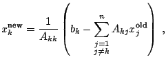
The intuition of the Jacobi method is very simple: given an approximation $\boldsymbol{x}^{\text{old}}$ of the solution, let us express the $k$th component $x_k$ of $\boldsymbol {x}$ as a function of the other components from the $k$th equation and compute $x_k$ given  $\boldsymbol{x}^{\text{old}}$:

$$x^{\text{new}}_k = \frac{1}{A_{kk}} \left(b_k - \sum^n_{\stackrel{\scriptstyle j=1}{j\neq k}} A_{kj} x^{\text{old}}_j\right)\;,$$ (4.11)

$k = 1,\ldots,n$ (see Fig. 4.4).

The Jacobi method converges for any starting vector $\boldsymbol{x}_0$ as long as $\rho(\boldsymbol{D}^{-1}(\boldsymbol{L}+\boldsymbol{U})) < 1$, see Theorem 7. This condition is satisfied for a relatively big class of matrices including diagonally dominant matrices (matrices $\boldsymbol{A}$ such that $\sum_{j=1,j\neq i}^n \vert A_{ij}\vert \leq \vert A_{ii}\vert$ for $i=1,\ldots,n$), and symmetric matrices $\boldsymbol{A}$ such that $\boldsymbol{D}$, $\boldsymbol{A}=\boldsymbol{L}+\boldsymbol{D}+\boldsymbol{U}$, and $-\boldsymbol{L}+\boldsymbol{D}-\boldsymbol{U}$ are all positive definite. Although there are many improvements to the basic principle of the Jacobi method in terms of convergence to $\boldsymbol{x}_{e}$, see Sects. 4.3.3 and 4.3.4, its advantage is an easy and fast implementation (elements of a new iteration $\boldsymbol{x}_i$ can be computed independently of each other).

4.3.3 Gauss-Seidel Method

Analogously to the Jacobi method, we can rewrite system (4.6) as $(\boldsymbol{L}+\boldsymbol{D})\boldsymbol{x} + \boldsymbol{U}\boldsymbol{x} = \boldsymbol{b}$, which further implies $\boldsymbol{x} = (\boldsymbol{L}+\boldsymbol{D})^{-1}[-\boldsymbol{U}\boldsymbol{x} + \boldsymbol{b}]$. This leads to the iteration formula of the Gauss-Seidel method:

$$\boldsymbol{x}_{i+1} = -(\boldsymbol{L}+\boldsymbol{D})^{-1}\boldsymbol{U}\boldsymbol{x}_i + (\boldsymbol{L}+\boldsymbol{D})^{-1}\boldsymbol{b}\;.$$ (4.12)

The main difference to the Jacobi methods lies in a more efficient use of (4.11). When computing the $k$th element $x_k^{\text{new}}$, the first $k-1$ elements $x_1^{\text{new}},\ldots,x_{k-1}^{\text{new}}$ are already known (and presumably more precise than $x_1^{\text{old}},\ldots,x_{k-1}^{\text{old}}$). Thus, it is possible to use these new values instead of the old ones and speed up the convergence (see Fig. 4.5 for a scheme). Moreover, using this strategy, the newly computed elements of $\boldsymbol{x}_{i+1}$ can directly overwrite the respective elements of $\boldsymbol{x}_i$ and save memory this way.

Figure 4.5: Scheme of the Gauss-Seidel method

Following the Theorem 7, the Gauss-Seidel method converges for any starting vector $\boldsymbol{x}_0$ if $\rho((\boldsymbol{L}+\boldsymbol{D})^{-1}\boldsymbol{U}) < 1$. This condition holds, for example, for diagonally dominant matrices as well as for positive definite ones.

4.3.4 Successive Overrelaxation Method

The successive overrelaxation (SOR) method aims to further refine the Gauss-Seidel method. The Gauss-Seidel formula (4.12) can be rewritten as

$$\boldsymbol{x}_{i+1} = \boldsymbol{x}_i - \boldsymbol{D}^{-1} [ \... ... - \boldsymbol{b}] = \boldsymbol{x}_i - \boldsymbol{\Delta}_{\boldsymbol{i}}\;,$$

which describes the difference $\boldsymbol{\Delta}_{\boldsymbol{i}}$ between $\boldsymbol{x}_{i+1}$ and $\boldsymbol{x}_i$ expressed for the $k$th element of $\boldsymbol{x}_{i(+1)}$ from the $k$th equation, $k = 1,\ldots,n$. The question SOR poses is whether the method can converge faster if we ''overly'' correct $\boldsymbol{x}_{i+1}$ in each step; that is, if $\boldsymbol{x}_i$ is corrected by a multiple $\omega$ of $\boldsymbol{\Delta}_{\boldsymbol{i}}$ in each iteration. This idea leads to the SOR formula:

$$\boldsymbol{x}_{i+1} = \boldsymbol{x}_i - \omega \boldsymbol{D}^{... ...i+1} + (\boldsymbol{D}+\boldsymbol{U}) \boldsymbol{x}_i \} - \boldsymbol{b}]\;,$$

or in the form (4.10),

$$\boldsymbol{x}_{i+1} = (\boldsymbol{D}+\omega\boldsymbol{L})^{-1}... ...symbol{x}_i + \omega(\boldsymbol{D}+\omega\boldsymbol{L})^{-1}\boldsymbol{b}\;.$$ (4.13)

The parameter $\omega$ is called the (over)relaxation parameter and it can be shown that SOR converges only for $\omega \in (0,2)$, a result derived by [41].

A good choice of parameter $\omega$ can speed up convergence, as measured by the spectral radius of the corresponding iteration matrix $\boldsymbol{B}$ (see Theorem 7; a lower spectral radius $\rho(\boldsymbol{B})$ means faster convergence). There is a choice of literature devoted to the optimal setting of relaxation parameter: see [28] for a recent overview of the main results concerning SOR. We just present one important result, which is due to [66].

Definition 1   A matrix $\boldsymbol{A}$ is said to be two-cyclic consistently ordered if the eigenvalues of the matrix $\boldsymbol{M}(\alpha) = \alpha\boldsymbol{D}^{-1}\boldsymbol{L} + \alpha^{-1}\boldsymbol{D}^{-1}\boldsymbol{U}$, $\alpha\neq 0$, are independent of $\alpha$.

Theorem 8   Let the matrix $\boldsymbol{A}$ be two-cyclic consistently ordered. Let the respective Gauss-Seidel iteration matrix $\boldsymbol{B} = -(\boldsymbol{L}+\boldsymbol{D})^{-1}\boldsymbol{U}$ have the spectral radius $\rho(\boldsymbol{B}) < 1$. Then the optimal relaxation parameter $\omega$ in SOR is given by

$$\omega_{\text{opt}} = \frac{2}{1+\sqrt{1-\rho(\boldsymbol{B})}}$$

and for this optimal value it holds $\rho(\boldsymbol{B};\omega_{\text{opt}}) = \omega_{\text{opt}} - 1$.

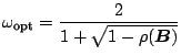Using SOR with the optimal relaxation parameter significantly increases the rate of convergence. Note however that the convergence acceleration is obtained only for $\omega$ very close to $\omega_{\text{opt}}$. If $\omega_{\text{opt}}$ cannot be computed exactly, it is better to take $\omega$ slightly larger rather than smaller. [24] describe an approximation algorithm for  $\rho(\boldsymbol{B})$.

On the other hand, if the assumptions of Theorem 8 are not satisfied, one can employ the symmetric SOR (SSOR), which performs the SOR iteration twice: once as usual, see (4.13), and once with interchanged $\boldsymbol{L}$ and  $\boldsymbol{U}$. SSOR requires more computations per iteration and usually converges slower, but it works for any positive definite matrix and can be combined with various acceleration techniques. See [7] and [28] for details.

4.3.5 Gradient Methods

Gradient iterative methods are based on the assumption that $\boldsymbol{A}$ is a symmetric positive definite matrix  $\boldsymbol{A}$. They use this assumption to reformulate (4.6) as a minimization problem: $\boldsymbol{x}_{e}$ is the only minimum of the quadratic form

$$Q(\boldsymbol{x}) = \frac{1}{2}\boldsymbol{x}^{\top} \boldsymbol{A} \boldsymbol{x} - \boldsymbol{x}^{\top} \boldsymbol{b}\;.$$

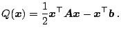Given this minimization problem, gradient methods construct an iteration series of vectors converging to $\boldsymbol{x}_{e}$ using the following principle. Having the $i$th approximation  $\boldsymbol{x}_i$, choose a direction $\boldsymbol{v}_i$ and find a number $\alpha_i$ such that the new vector

$$\boldsymbol{x}_{i+1} = \boldsymbol{x}_i + \alpha_i\boldsymbol{v}_i$$

is a minimum of $Q(\boldsymbol{x})$ on the line $\boldsymbol{x}_i + \alpha\boldsymbol{v}_i$, $\alpha \in {\mathbb{R}}$. Various choices of directions $\boldsymbol{v}_i$ then render different gradient methods, which are in general nonstationary ( $\boldsymbol{v}_i$ changes in each iteration). We discuss here three methods: the Gauss-Seidel (as a gradient method), steepest descent and conjugate gradients methods.

4.3.5.1 Gauss-Seidel Method as a Gradient Method

Interestingly, the Gauss-Seidel method can be seen as a gradient method for the choice

$$\boldsymbol{v}_{kn+i} = \boldsymbol{e}_i\;, \quad k=0,1,2,\ldots\;, \quad i=1,\ldots,n\;,$$

where $\boldsymbol{e}_i$ denotes the $i$th unit vector. The $k$th Gauss-Seidel iteration corresponds to $n$ subiterations with $\boldsymbol{v}_{kn+i}$ for $i=1,\ldots,n$.

4.3.5.2 Steepest Descent Method

The steepest descent method is based on the direction $\boldsymbol{v}_i$ given by the gradient of $Q(\boldsymbol{x})$ at $\boldsymbol{x}_i$. Denoting the residuum of the $i$th approximation $\boldsymbol{r}_i = \boldsymbol{b} - \boldsymbol{A} \boldsymbol{x}_i$, the iteration formula is

$$\boldsymbol{x}_{i+1} = \boldsymbol{x}_i + \frac{\boldsymbol{r}_i^... ...i}{\boldsymbol{r}_i^{\top} \boldsymbol{A} \boldsymbol{r}_i} \boldsymbol{r}_i\;,$$

where $\boldsymbol{r}_i$ represents the direction $\boldsymbol{v}_i$ and its coefficient is the $Q(\boldsymbol{x})$-minimizing choice of $\alpha_i$. By definition, this method reduces $Q(\boldsymbol{x}_i)$ at each step, but it is not very effective. The conjugate gradient method discussed in the next subsection will usually perform better.

4.3.5.3 Conjugate Gradient Method

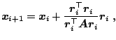In the conjugate gradient (CG) method proposed by [33], the directions $\boldsymbol{v}_i$ are generated by the $\boldsymbol{A}$-orthogonalization of residuum vectors. Given a symmetric positive definite matrix  $\boldsymbol{A}$, $\boldsymbol{A}$-orthogonalization is a procedure that constructs a series of linearly independent vectors $\boldsymbol{v}_i$ such that $\boldsymbol{v}_i^{\top} \boldsymbol{A} \boldsymbol{v}_j = 0$ for $i\neq j$ (conjugacy or $\boldsymbol{A}$-orthogonality condition). It can be used to solve the system (4.6) as follows ( $\boldsymbol{r}_i = \boldsymbol{b} - \boldsymbol{A} \boldsymbol{x}_i$ represents residuals).

Algorithm 8    
$\boldsymbol{v}_0 = \boldsymbol{r}_0 = \boldsymbol{b} - \boldsymbol{A}\boldsymbol{x}_0$
do
     $\alpha_{i~~~\!} = {\left(\boldsymbol{v}_i^{\top} \boldsymbol{r}_i\right)} / {\left(\boldsymbol{v}_i^{\top} \boldsymbol{A} \boldsymbol{v}_i\right)}$
     $\boldsymbol{x}_{i+1} = \boldsymbol{x}_i + \alpha_i \boldsymbol{v}_i$
     $\boldsymbol{r}_{i+1\,} = \boldsymbol{r}_i - \alpha_i \boldsymbol{A} \boldsymbol{v}_i$
     $\beta_{i~~~\,} = -{\left(\boldsymbol{v}_i^{\top} \boldsymbol{A} \boldsymbol{r}... ...ight)} / {\left(\boldsymbol{v}_i^{\top} \boldsymbol{A} \boldsymbol{v}_i\right)}$
     $\boldsymbol{v}_{i+1} = \boldsymbol{r}_{i+1} + \beta_i \boldsymbol{v}_i$
until a stop criterion holds

An interesting theoretic property of CG is that it reaches the exact solution in at most $n$ steps because there are not more than $n$ ( $\boldsymbol{A}$-)orthogonal vectors. Thus, CG is not a truly iterative method. (This does not have to be the case if $\boldsymbol{A}$ is a singular or non-square matrix, see [42].) On the other hand, it is usually used as an iterative method, because it can give a solution within the given accuracy much earlier than after $n$ iterations. Moreover, if the approximate solution $\boldsymbol{x}_n$ after $n$ iterations is not accurate enough (due to computational errors), the algorithm can be restarted with $\boldsymbol{x}_0$ set to  $\boldsymbol{x}_n$. Finally, let us note that CG is attractive for use with large sparse matrices because it addresses $\boldsymbol{A}$ only by its multiplication by a vector. This operation can be done very efficiently for a properly stored sparse matrix, see Sect. 4.5.

The principle of CG has many extensions that are applicable also for nonsymmetric nonsingular matrices: for example, generalized minimal residual, [55]; (stabilized) biconjugate gradients, [64]; or quasi-minimal residual, [13].