Subsections

• 7.4.1 The Cascade Algorithm
• 7.4.2 Matlab Implementation of Cascade Algorithm

7.4 Discrete Wavelet Transforms

Discrete wavelet transforms (DWT) are applied to discrete data sets and produce discrete outputs. Transforming signals and data vectors by DWT is a process that resembles the fast Fourier transform (FFT), the Fourier method applied to a set of discrete measurements.

Table 7.2: The analogy between Fourier and wavelet methods

Fourier Methods	Fourier Integrals	Fourier Series	Discrete Fourier Transforms
Wavelet Methods	Continuous Wavelet Transforms	Wavelet Series	Discrete Wavelet Transforms

The analogy between Fourier and wavelet methods is even more complete (Table 7.2) when we take into account the continuous wavelet transform and wavelet series expansions.

Discrete wavelet transforms map data from the time domain (the original or input data vector) to the wavelet domain. The result is a vector of the same size. Wavelet transforms are linear and they can be defined by matrices of dimension $n \times n$ if they are applied to inputs of size $n$. Depending on boundary conditions, such matrices can be either orthogonal or ''close'' to orthogonal. When the matrix is orthogonal, the corresponding transform is a rotation in  ${{\mathbb{R}}}^n$ in which the data (a $n$-typle) is a point in  ${{\mathbb{R}}}^n$. The coordinates of the point in the rotated space comprise the discrete wavelet transform of the original coordinates. Here we provide two toy examples.

Example 5   Let the vector be $(1,2)$ and let $M(1,2)$ be the point in ${{\mathbb{R}}}^2$ with coordinates given by the data vector. The rotation of the coordinate axes by an angle of $\pi/4$ can be interpreted as a DWT in the Haar wavelet basis. The rotation matrix is

$$W = \left( \begin{array}{cc} \cos \frac{\pi}{4} & \sin \frac{\pi}... ...1}{\sqrt{2}} \\ \frac{1}{\sqrt{2}} & -\frac{1}{\sqrt{2}} \end{array} \right){},$$

and the discrete wavelet transform of $(1,2)'$ is $W \cdot (1,2)' = (3/\sqrt{2}, -1/\sqrt{2})'$. Notice that the energy (squared distance of the point from the origin) is preserved, $1^2 + 2^2 = (1/2)^2 + (\sqrt{3}/2)^2$, since $W$ is a rotation.

Example 6   Let ${\boldsymbol{y} }= (1,0,-3,2,1,0,1,2)$. The associated function $f$ is given in Fig. 7.10. The values $f(n) = y_n,~ n = 0, 1, \ldots, 7$ are interpolated by a piecewise constant function. We assume that $f$ belongs to Haar's multiresolution space $V_0$.

Figure 7.10: A function interpolating $\boldsymbol {y}$ on $[0,8)$

The following matrix equation gives the connection between $\boldsymbol {y}$ and the wavelet coefficients (data in the wavelet domain).

$$\left[ \begin{array}{c} 1 \\ 0 \\ -3 \\ 2 \\ 1 \\ 0 \\ 1 \\ 2 \en... ...d_{10} \\ d_{11} \\ d_{20} \\ d_{21} \\ d_{22} \\ d_{23} \end{array} \right]{}.$$

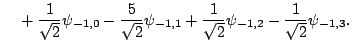
The solution is

$$\left[ \begin{array}{c} c_{00} \\ d_{00} \\ d_{10} \\ d_{11} \\ d... ...{\sqrt{2}} \\ \frac{1}{\sqrt{2}} \\ -\frac{1}{\sqrt{2}} \end{array} \right] {}.$$

Thus,

$$f = \sqrt{2} \phi_{-3,0} - \sqrt{2} \psi_{-3,0} + \psi_{-2,0} - \psi_{-2,1}$$

$$\quad{}+\frac{1}{\sqrt{2}} \psi_{-1,0} -\frac{5}{\sqrt{2}} \psi_{-1,1} +\frac{1}{\sqrt{2}} \psi_{-1,2} -\frac{1}{\sqrt{2}} \psi_{-1,3}{}.$$ (7.45)

The solution is easy to verify. For example, when $x \in [0,1)$,

$$f(x) = \sqrt{2} \cdot \frac{1}{2 \sqrt{2}} - \sqrt{2} \cdot \frac... ...1}{\sqrt{2}} \cdot \frac{1}{\sqrt{2}} = \frac{1}{2} + \frac{1}{2} = 1~(=y_0){}.$$

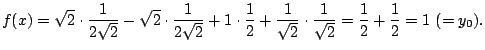Applying wavelet transforms by multiplying the input vector with an appropriate orthogonal matrix is conceptually straightforward task, but of limited practical value. Storing and manipulating the transformation matrices for long inputs $( n > 2000)$ may not even be feasible.

This obstacle is solved by the link of discrete wavelet transforms with fast filtering algorithms from the field of signal and image processing.

7.4.1 The Cascade Algorithm

Mallat (1989a,b)[16,17] was the first to link wavelets, multiresolution analyses and cascade algorithms in a formal way. Mallat's cascade algorithm gives a constructive and efficient recipe for performing the discrete wavelet transform. It relates the wavelet coefficients from different levels in the transform by filtering with wavelet filter $\boldsymbol{h}$ and and its mirror counterpart  $\boldsymbol{g}$.

It is convenient to link the original data with the space $V_J$, where $J$ is often 0 or $\log n$, where $n$ is a dyadic size of data. Then, coarser smooth and complementing detail spaces are $(V_{J-1}, W_{J-1})$, $(V_{J-2}, W_{J-2})$, etc. Decreasing the index in $V$-spaces is equivalent to coarsening the approximation to the data.

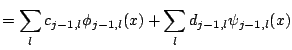
By a straightforward substitution of indices in the scaling equations (7.21) and (7.35), one obtains

$$\phi_{j-1,l}(x) = \sum_{k \in {{\mathbb{Z}}}} h_{k-2l} \phi_{jk}(... ...nd}\quad \psi_{j-1,l}(x) = \sum_{k \in {{\mathbb{Z}}}} g_{k-2l} \phi_{jk}(x){}.$$ (7.46)

The relations in (7.46) are fundamental in developing the cascade algorithm.

In a multiresolution analysis, $\ldots \subset V_{j-1} \subset V_j \subset V_{j+1} \subset \ldots$. Since $V_j = V_{j-1} \oplus W_{j-1}$, any function $v_j \in V_j$ can be represented uniquely as $v_j(x) = v_{j-1}(x) + w_{j-1}(x)$, where $v_{j-1} \in V_{j-1}$ and $w_{j-1} \in W_{j-1}$. It is customary to denote the coefficients associated with $\phi_{jk}(x)$ and $\psi_{jk}(x)$ by $c_{jk}$ and $d_{jk}$, respectively.

Thus,

$$v_j(x) = \sum_{k} c_{j,k} \phi_{j,k}(x)$$

$$= \sum_{l} c_{j-1,l} \phi_{j-1,l}(x) + \sum_{l} d_{j-1,l} \psi_{j-1,l}(x)$$

$$= v_{j-1}(x) + w_{j-1} (x){}.$$

By using the general scaling equations (7.46), orthogonality of $w_{j-1}(x)$ and $\phi_{j-1, l}(x)$ for any $j$ and $l$, and additivity of inner products, we obtain

$$c_{j-1,l} = \langle v_j, \phi_{j-1, l} \rangle$$

$$= \left\langle v_j, \sum_{k} h_{k - 2l} \phi_{j, k} \right\rangle$$

$$= \sum_{k} h_{k - 2l} \langle v_j, \phi_{j,k} \rangle$$ (7.47)

$$= \sum_{k} h_{k - 2l} c_{j, k}{}.$$

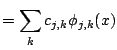Similarly $d_{j-1, l} = \sum_k g_{k-2l} c_{j,k}$.

The cascade algorithm works in the reverse direction as well. Coefficients in the next finer scale corresponding to $V_j$ can be obtained from the coefficients corresponding to $V_{j-1}$ and $W_{j-1}$. The relation

$$c_{j,k} = \langle v_j, \phi_{j, k} \rangle$$

$$= \sum_l c_{j-1,l} \langle \phi_{j-1, l}, \phi_{j,k}\rangle + \sum_l d_{j-1,l} \langle \psi_{j-1, l}, \phi_{j,k}\rangle$$ (7.48)

$$= \sum_l c_{j-1,l} h_{k-2l} + \sum_l d_{j-1,l} g_{k-2l}{},$$

describes a single step in the reconstruction algorithm.

The discrete wavelet transform can be described in terms of operators. Let the operators  ${\mathcal{H}}$ and  ${\mathcal{G}}$ acting on a sequence $a=\{ a_n, n \in {{\mathbb{Z}}}\}$, satisfy the following coordinate-wise relations:

$$({\mathcal{H}} a)_k = \sum_n h_{n - 2 k} a_n\quad ({\mathcal{G}} a)_k = \sum_n g_{n - 2 k} a_n{},$$

and their adjoint operators ${\mathcal{H}}^{\ast}$ and ${\mathcal{G}}^{\ast}$ satisfy:

$$({{\mathcal{H}}^{\ast}} a)_n = \sum_k h_{n - 2 k} a_k\quad ({{\mathcal{G}}^{\ast}} a)_n = \sum_k g_{n - 2 k} a_k{},$$

where ${\boldsymbol{h}}=\{h_n\}$ is wavelet filter and ${\boldsymbol{g}}=\{g_n\}$ its quadrature-mirror counterpart.

Denote the original signal by ${\boldsymbol{c}}^{(J)}=\{c^{(J)}_k\}$. If the signal is of length $2^J$, then ${\boldsymbol{c}}^{(J)}$ can be interpolated by the function $f(x) = \sum c^{(J)}_k \phi (x-k)$ from $V_J$. In each step of the wavelet transform, we move to the next coarser approximation (level) ${\boldsymbol{c}}^{(\kern.5pt j-1)}$ by applying the operator  ${\mathcal{H}}$, ${\boldsymbol{c}}^{(j-1)} = {\mathcal{H}} {\boldsymbol{c}}^{(j)}$. The ''detail information,'' lost by approximating ${\boldsymbol{c}}^{(j)}$ by the ''averaged'' ${\boldsymbol{c}}^{(j-1)}$, is contained in vector ${\boldsymbol{d}}^{(j-1)} = {\mathcal{G}} {\boldsymbol{c}}^{(j)}$.

The discrete wavelet transform of a sequence $\boldsymbol{y} = {\boldsymbol{c}}^{(J)}$ of length $2^J$ can then be represented as

$$\left({\boldsymbol{c}}^{(J-k)},{\boldsymbol{d}}^{(J-k)}, {\boldsy... ...(J-k+1)}, \ldots, {\boldsymbol{d}}^{(J-2)}, {\boldsymbol{d}}^{(J-1)} \right){}.$$ (7.49)

Notice that the lengths of $\boldsymbol {y}$ and its transform in (7.49) coincide. Because of decimation, the length of ${\boldsymbol{c}}^{(j)}$ is twice the length of ${\boldsymbol{c}}^{(j-1)}$, and $2^J = 2^{J-k} + \sum_{i=1}^k 2^{J-i}$, $1 \leq k \leq J$.

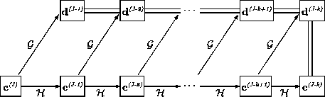
For an illustration of (7.49), see Fig. 7.11. By utilizing the operator notation, it is possible to summarize the discrete wavelet transform (curtailed at level $k$) in a single line:

$${\boldsymbol{y}} \mapsto \left({\mathcal{H}}^{k} {\boldsymbol{y}}... ...al{G}} {\mathcal{H}} {\boldsymbol{y}},{\mathcal{G}} {\boldsymbol{y}} \right){}.$$

The number $k$ can be any arbitrary integer between $1$ and $J$ and it is associated with the coarsest ''smooth'' space, $V_{J-k}$, up to which the transform was curtailed. In terms of multiresolution spaces, (7.49) corresponds to the multiresolution decomposition $V_{J-k} \oplus W_{J-k} \oplus W_{J-k+1} \oplus \ldots \oplus W_{J-1}$. When $k=J$ the vector ${\boldsymbol{c}}^{(0)}$ contains a single element, $c^{(0)}$.

Figure 7.11: Forward wavelet transform of depth $k$ (DWT is a vector of coefficients connected by double lines)

If the wavelet filter length exceeds $2$, one needs to define actions of the filter beyond the boundaries of the sequence to which the filter is applied. Different policies are possible. The most common is a periodic extension of the original signal.

The reconstruction formula is also simple in terms of operators ${\mathcal{H}}^{\ast}$ and ${\mathcal{G}}^{\ast}$. They are applied on ${\boldsymbol{c}}^{(\kern.5pt j-1)}$ and ${\boldsymbol{d}}^{(\kern.5pt j-1)}$, respectively, and the results are added. The vector ${\boldsymbol{c}}^{(\kern.5pt j)}$ is reconstructed as

$${\boldsymbol{c}}^{(\kern.5pt j)} = {\mathcal{H}}^{\ast} {\boldsym... ...^{(\kern.5pt j-1)} + {\mathcal{G}}^{\ast} {\boldsymbol{d}}^{(\kern.5pt j-1)}{},$$ (7.50)

Recursive application of (7.50) leads to

$$\left({\mathcal{H}}^{k} {\boldsymbol{y}}, {\mathcal{G}} {\mathcal... ...\mathcal{G}} {\mathcal{H}}{\boldsymbol{y}},{\mathcal{G}}{\boldsymbol{y}}\right)$$

$$= \left({\boldsymbol{c}}^{(J-k)}, {\boldsymbol{d}}^{(J-k)}, {\bol... ...d}}^{(J-k+1)},\ldots, {\boldsymbol{d}}^{(J-2)}, {\boldsymbol{d}}^{(J-1)}\right)$$

$$\mapsto \sum_{i=1}^{k-1} \left({\mathcal{H}}^{\ast}\right)^{k-1-i... ...t({\mathcal{H}}^{\ast} \right)^k {\boldsymbol{c}}^{(J-k)} = {\boldsymbol{y}}{}.$$

Figure 7.12: Inverse Transform

Example 7   Let ${\boldsymbol{y} }= (1,0,-3,2,1,0,1,2)$ be an exemplary set we want to transform by Haar's DWT. Let $k=J=3$, i.e., the coarsest approximation and detail levels will contain a single point each. The decomposition algorithm applied on ${\boldsymbol{y} }= (1,0,-3,2,1,0,1,2)$ is given schematically in Fig. 7.13.

Figure 7.13: An illustration of a decomposition procedure

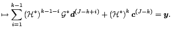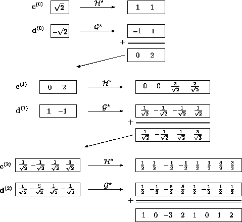
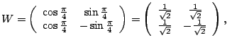
For the Haar wavelet, the operators ${\mathcal{H}}$ and ${\mathcal{G}}$ are given by $({\mathcal{H}} a)_k = \sum_n h_{n-2k} a_n= \sum_m h_m a_{m+2k} = h_0 a_{2k} + h_1 a_{2k+1}= (a_{2k}+ a_{2k+1})/{\sqrt{2}}$. Similarly, $({\mathcal{G}} a)_k = \sum_n g_{n-2k} a_n= \sum_m g_m a_{m+2k} = g_0 a_{2k} + g_1 a_{2k+1}= (a_{2k} - a_{2k+1})/{\sqrt{2}}$.

Figure 7.14: An illustration of a reconstruction procedure

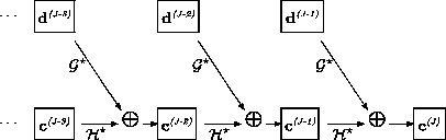
The reconstruction algorithm is given in Fig. 7.14. In the process of reconstruction, $({\mathcal{H}}^{\ast} a)_n = \sum_k h_{n-2k} a_k$, and $({\mathcal{G}}^{\ast} a)_n = \sum_k g_{n-2k} a_k$. For instance, the first line in Fig. 7.14 recovers the object $\{1,1\}$ from $\sqrt{2}$ by applying ${\mathcal{H}}^{\ast}$. Indeed, $({\mathcal{H}}^{\ast} \{a_0\})_0 = h_0 \sqrt{2} = 1$ and $({\mathcal{H}}^{\ast} \{a_0\})_1 = h_1 \sqrt{2} = 1$.

We already mentioned that when the length of the filter exceeds 2, boundary problems occur since the convolution goes outside the range of data.

There are several approaches to resolving the boundary problem. The signal may be continued in a periodic way ( $\ldots, y_{n-1}, y_n \vert y_1, y_2, \ldots$), symmetric way ( $\ldots, y_{n-1},y_n \vert y_{n-1}, y_{n-2}, \ldots$), padded by a constant, or extrapolated as a polynomial. Wavelet transforms can be confined to an interval (in the sense of Cohen, Daubechies and Vial (1993)[7] and periodic and symmetric extensions can be viewed as special cases. Periodized wavelet transforms are also defined in a simple way.

If the length of the data set is not a power of $2$, but of the form $M \cdot 2^K$, for $M$ odd and $K$ a positive integer, then only $K$ steps in the decomposition algorithm can be performed. For precise descriptions of conceptual and calculational hurdles caused by boundaries and data sets whose lengths are not a power of 2, we direct the reader to the monograph by Wickerhauser (1994)[26].

In this section we discussed the most basic wavelet transform. Various generalizations include biorthogonal wavelets, multiwavelets, nonseparable multidimensional wavelet transforms, complex wavelets, lazy wavelets, and many more.

For various statistical applications of wavelets (nonparametric regression, density estimation, time series, deconvolutions, etc.) we direct the reader to Antoniadis (1997)[2], Härdle et al. (1998)[15], Vidakovic (1999)[23]. An excellent monograph by Walter and Shen (2000)[25] discusses statistical applications of wavelets and various other orthogonal systems.

7.4.2 Matlab Implementation of Cascade Algorithm

The following two matlab m-files implement discrete wavelet transform and its inverse, with periodic handling of boundaries. The data needs to be of dyadic size (power of $2$). The programs are didactic, rather than efficient. For an excellent and comprehensive wavelet package, we direct the reader to wavelab802 module (http://www-stat.stanford.edu/~ wavelab/) maintained by Donoho and his coauthors.

function dwtr = dwtr(data, L, filterh)
%  function dwtr = dwt(data, filterh, L);
%  Calculates the DWT of periodic data set
%  with scaling filter  filterh  and  L  scales.
%
%   Example of Use:
%   data = [1 0 -3 2 1 0 1 2]; filter = [sqrt(2)/2 sqrt(2)/2];
%   wt = DWTR(data, 3, filter)
%------------------------------------------------------------------

n = length(filterh);                %Length of wavelet filter
C = data;                           %Data \qut{live} in V_J
dwtr = [];                          %At the beginning dwtr empty
H  =  fliplr(filterh);              %Flip because of convolution
G  =  filterh;                      %Make quadrature mirror
G(1:2:n) = -G(1:2:n);               %    counterpart
for j = 1:L                         %Start cascade
  nn = length(C);                   %Length needed to
  C = [C(mod((-(n-1):-1),nn)+1) C]; % make periodic
  D = conv(C,G);                    %Convolve,
  D = D([n:2:(n+nn-2)]+1);          %  keep periodic, decimate
  C = conv(C,H);                    %Convolve,
  C = C([n:2:(n+nn-2)]+1);          %  keep periodic, decimate
  dwtr = [D,dwtr];                  %Add detail level to dwtr
end;                                %Back to cascade or end
dwtr = [C, dwtr];                   %Add the last \qut{smooth} part

function  data = idwtr(wtr, L, filterh)
% function data = idwt(wtr, L, filterh);
% Calculates the IDWT of wavelet
% transform wtr using wavelet filter
% \qut{filterh}  and  L  scales.
% Example:
%>> max(abs(data - IDWTR(DWTR(data,3,filter), 3,filter)))
%ans = 4.4409e-016
%----------------------------------------------------------------
nn = length(wtr);   n = length(filterh); %Lengths
if nargin==2, L = round(log2(nn)); end;  %Depth of transform
H = filterh;                             %Wavelet H filter
G = fliplr(H); G(2:2:n) = -G(2:2:n);     %Wavelet G filter
LL = nn/(2^L);                           %Number of scaling coeffs
C =  wtr(1:LL);                          %Scaling coeffs
for j = 1:L                              %Cascade algorithm
   w  = mod(0:n/2-1,LL)+1;               %Make periodic
   D  = wtr(LL+1:2*LL);                  %Wavelet coeffs
   Cu(1:2:2*LL+n) = [C C(1,w)];          %Upsample & keep periodic
   Du(1:2:2*LL+n) = [D D(1,w)];          %Upsample & keep periodic
   C  = conv(Cu,H) + conv(Du,G);         %Convolve & add
   C  = C([n:n+2*LL-1]-1);               %Periodic part
   LL = 2*LL;                            %Double the size of level
end;
data = C;                                %The inverse DWT