We illustrate in this section that model selection boils down to compromises between different aspects of a model. Occam's razor has been the guiding principle for the compromises: the model that fits observations sufficiently well in the least complex way should be preferred. Formalization of this principle is, however, nontrivial.
To be precise on fits observations sufficiently well, one needs a quantity that measures how well a model fits the data. This quantity is often called the goodness-of-fit (GOF). It usually is the criterion used for estimation, after deciding on a model. For example, we have used the LS as a measure of the GOF for regression models in Sect. 1.1. Other GOF measures include likelihood for density estimation problems and classification error for pattern recognition problems.
To be precise on the least complex way, one needs
a quantity that measures the complexity of a model. For
a parametric model, a common measure of model complexity is
the number of parameters in the model, often called the
degrees of freedom (df). For
a non-parametric regression model like the periodic spline,
![]() , a direct extension from its parametric
version, is often used as a measure of model complexity
([24]).
, a direct extension from its parametric
version, is often used as a measure of model complexity
([24]).
![]() will also be
refered to as the degrees of freedom. The middle panel of
Fig. 1.3 depicts how
will also be
refered to as the degrees of freedom. The middle panel of
Fig. 1.3 depicts how
![]() for the
periodic spline depends on the smoothing parameter
for the
periodic spline depends on the smoothing parameter ![]() .
Since there is an one-to-one correspondence between
.
Since there is an one-to-one correspondence between ![]() and
and
![]() , both of them are used as model index
([24]). See [21] for discussions on
some subtle issues concerning model index for smoothing spline
models. For some complicated models such as tree-based
regression, there may not be an obvious measure of model
complexity ([58]). In these cases the generalized
degrees of freedom defined
in [58] may be used. Section 1.3
contains more details on the generalized degrees of freedom.
, both of them are used as model index
([24]). See [21] for discussions on
some subtle issues concerning model index for smoothing spline
models. For some complicated models such as tree-based
regression, there may not be an obvious measure of model
complexity ([58]). In these cases the generalized
degrees of freedom defined
in [58] may be used. Section 1.3
contains more details on the generalized degrees of freedom.
To illustrate the interplay between the GOF and model
complexity, we fit trigonometric regression models from the
smallest model with ![]() to the largest model with
to the largest model with
![]() . The square root of residual sum of squares (RSS)
are plotted against the degrees of freedom (
. The square root of residual sum of squares (RSS)
are plotted against the degrees of freedom (
![]() ) as
circles in the left panel of Fig. 1.3.
Similarly, we fit the periodic spline with a wide range of
values for the smoothing parameter
) as
circles in the left panel of Fig. 1.3.
Similarly, we fit the periodic spline with a wide range of
values for the smoothing parameter ![]() . Again, we plot
the square root of RSS against the degrees of freedom
(
. Again, we plot
the square root of RSS against the degrees of freedom
(
![]() ) as the solid line in the left panel of
Fig. 1.3. Obviously, RSS decreases to zero
(interpolation) as the degrees of freedom increases to
) as the solid line in the left panel of
Fig. 1.3. Obviously, RSS decreases to zero
(interpolation) as the degrees of freedom increases to
![]() . RSS keeps declining almost linearly after the initial big
drop. It is quite clear that the constant model does not fit
data well. But it is unclear which model fits
observations sufficiently well.
. RSS keeps declining almost linearly after the initial big
drop. It is quite clear that the constant model does not fit
data well. But it is unclear which model fits
observations sufficiently well.
![\includegraphics[width=\textwidth,clip]{text/3-1/ssr.eps}](img3292.gif)
|
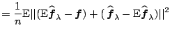
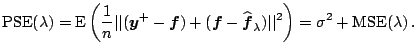
The previous example shows that the GOF and complexity are two opposite aspects of a model: the approximation error decreases as the model complexity increases. On the other hand, the Occam's razor suggests that simple models should be preferred to more complicated ones, other things being equal. Our goal is to find the ''best'' model that strikes a balance between these two conflicting aspects. To make the word ''best'' meaningful, one needs a target criterion which quantifies a model's performance. It is clear that the GOF cannot be used as the target because it will lead to the most complex model. Even though there is no universally accepted measure, some criteria are widely accepted and used in practice. We now discuss one of them which is commonly used for regression models.
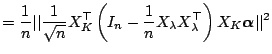
Let
![]() be an estimate of the function in
model (1.2) based on the model space
be an estimate of the function in
model (1.2) based on the model space
![]() . Let
. Let
![]() and
and
![]() . Define the
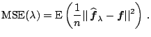
mean squared error (MSE) by
. Define the
mean squared error (MSE) by
 |
Another closely related target criterion is the average predictive squared error (PSE)
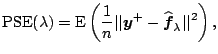 |
(1.16) |
 |
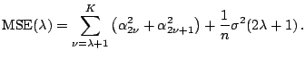
To illustrate the bias-variance trade-off,
we now calculate MSE for the
trigonometric regression and periodic spline models. For
notational simplicity, we assume that ![]() :
:
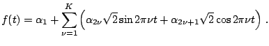 |
(1.17) |
Bias-Variance Trade-Off for the Trigonometric Regression.
![]() consists of the first
consists of the first
![]() columns of the
orthogonal matrix
columns of the
orthogonal matrix ![]() . Thus
. Thus
![]() .
.
![]() , where
, where
![]() consists of the first
consists of the first
![]() elements in
elements in
![]() . Thus
. Thus
![]() is unbiased. Furthermore,
is unbiased. Furthermore,
 |
||
 |
||
 |
||
 |
||
 |
 |
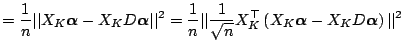
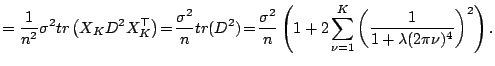
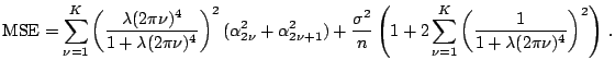
Bias-Variance Trade-Off for Periodic Spline.
For the
approximate periodic spline estimator, it is easy to check
that
![]() ,
,
![]() ,
,
![]() ,
,
![]() ,
,
![]() , and
, and
![]() . Thus all coefficients are shrunk to zero
except
. Thus all coefficients are shrunk to zero
except
![]() which is unbiased. The amount of
shinkage is controlled by the smoothing parameter
which is unbiased. The amount of
shinkage is controlled by the smoothing parameter ![]() .
It is straightforward to calculate the
.
It is straightforward to calculate the
![]() and
and
![]() in (1.15).
in (1.15).
 |
||
 |
||
 |
 |
It is easy to see that as ![]() increases from zero to
infinity, the
increases from zero to
infinity, the
![]() increases from zero to
increases from zero to
![]() and the
and the
![]() decreases from
decreases from ![]() to
to
![]() .
.
To calculate
![]() , one needs to know the true function. We use
the following simulation for illustration. We generate
responses from model (1.2) with
, one needs to know the true function. We use
the following simulation for illustration. We generate
responses from model (1.2) with
![]() and
and
![]() . The same design points in the
climate data is used:
. The same design points in the
climate data is used:
![]() and
and ![]() . The
true function and responses are shown in the left panel of
Fig. 1.4. We compute
. The
true function and responses are shown in the left panel of
Fig. 1.4. We compute
![]() ,
,
![]() .
. ![]() represents the contribution from frequency
represents the contribution from frequency ![]() . In the
right panel of Fig. 1.4, we plot
. In the
right panel of Fig. 1.4, we plot ![]() against frequency
against frequency ![]() with the threshold,
with the threshold,
![]() , marked as the dashed line. Except for
, marked as the dashed line. Except for
![]() ,
, ![]() decreases as
decreases as ![]() increases. Values of
increases. Values of
![]() are above the threshold for the first four
frequencies. Thus the optimal choice is
are above the threshold for the first four
frequencies. Thus the optimal choice is ![]() .
.
![\includegraphics[width=10.9cm,clip]{text/3-1/simdata.eps}](img3357.gif) |
![]() ,
,
![]() and
and
![]() are plotted against
frequency (
are plotted against
frequency (
![]() ) for trigonometric regression
(periodic spline) in the left (right) panel of
Fig. 1.5. Obviously, as the frequency
(
) for trigonometric regression
(periodic spline) in the left (right) panel of
Fig. 1.5. Obviously, as the frequency
(![]() ) increases (decreases), the
) increases (decreases), the
![]() decreases and the
decreases and the
![]() increases. The
increases. The
![]() represents
a balance between
represents
a balance between
![]() and
and
![]() . For the
trigonometric regression, the minimum of the
. For the
trigonometric regression, the minimum of the
![]() is reached at
is reached at
![]() , as expected.
, as expected.
![\includegraphics[width=10.9cm]{text/3-1/mse.eps}](img3359.gif) |
After deciding on a target criterion such as the
![]() , ideally
one would select the model to minimize this criterion. This
is, however, not practical because the criterion usually
involves some unknown quantities. For example,
, ideally
one would select the model to minimize this criterion. This
is, however, not practical because the criterion usually
involves some unknown quantities. For example,
![]() depends on
the unknown true function
depends on
the unknown true function ![]() which one wants to estimate in
the first place. Thus one needs to estimate this criterion
from the data and then minimize the estimated criterion. We
discuss unbiased and cross-validation estimates of
which one wants to estimate in
the first place. Thus one needs to estimate this criterion
from the data and then minimize the estimated criterion. We
discuss unbiased and cross-validation estimates of
![]() in
Sects 1.3 and 1.4
respectively.
in
Sects 1.3 and 1.4
respectively.