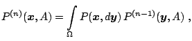
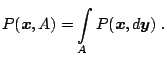
Markov chain Monte Carlo is a method to sample a given multivariate
distribution
![]() by constructing a suitable Markov chain
with the property that its limiting,
invariant distribution, is the target distribution
by constructing a suitable Markov chain
with the property that its limiting,
invariant distribution, is the target distribution
![]() . In
most problems of interest, the distribution
. In
most problems of interest, the distribution
![]() is absolutely
continuous and, as a result, the theory of MCMC methods is based on
that of Markov chains on continuous state spaces outlined, for
example, in [42] and [40]. [59] is the
fundamental reference for drawing the connections between this
elaborate Markov chain theory and MCMC methods. Basically, the goal of
the analysis is to specify conditions under which the constructed
Markov chain converges to the invariant distribution, and conditions
under which sample path averages based on the output of the Markov
chain satisfy a law of large numbers and a central limit theorem.
is absolutely
continuous and, as a result, the theory of MCMC methods is based on
that of Markov chains on continuous state spaces outlined, for
example, in [42] and [40]. [59] is the
fundamental reference for drawing the connections between this
elaborate Markov chain theory and MCMC methods. Basically, the goal of
the analysis is to specify conditions under which the constructed
Markov chain converges to the invariant distribution, and conditions
under which sample path averages based on the output of the Markov
chain satisfy a law of large numbers and a central limit theorem.
A
Markov chain is a collection of random variables (or vectors)
![]() where
where
![]() . The evolution of the Markov chain on a space
. The evolution of the Markov chain on a space
![]() is governed by the
transition kernel
is governed by the
transition kernel
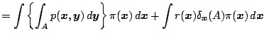
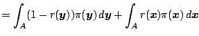
Generally, the transition kernel in Markov chain simulations has both
a continuous and discrete component. For some function
![]() , the
kernel can be expressed as
, the
kernel can be expressed as
The transition kernel is thus the distribution of
![]() given that
given that
![]() . The
. The
![]() th step ahead transition kernel is given by
th step ahead transition kernel is given by
 |
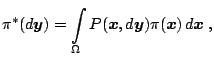
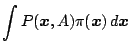
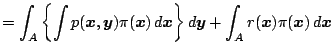
A Markov chain is
reversible if the function
![]() in (3.2)
satisfies
in (3.2)
satisfies
A minimal requirement on the Markov chain for it to satisfy a law of
large numbers is the requirement of
![]() -irreducibility. This
means that the chain is able to visit all sets with positive
probability under
-irreducibility. This
means that the chain is able to visit all sets with positive
probability under
![]() from any starting point in
from any starting point in ![]() .
Formally, a Markov chain is said to be
.
Formally, a Markov chain is said to be
![]() -irreducible if for every
-irreducible if for every
![]() ,
,
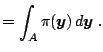
Another important property of a chain is aperiodicity, which ensures
that the chain does not cycle through a finite number of
sets. A Markov chain is
aperiodic if there exists no partition of
![]() for some
for some ![]() such that
such that
![]() for all
for all ![]() .
.
These definitions allow us to state the following results from
[59] which form the basis for Markov chain Monte Carlo
methods. The first of these results gives conditions under which
a strong law of large numbers holds and the second gives conditions
under which the probability density of the ![]() th iterate of the Markov
chain converges to its unique, invariant density.
th iterate of the Markov
chain converges to its unique, invariant density.
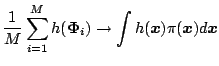 as as |
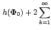
A further strengthening of the conditions is required to obtain
a central limit theorem for sample-path averages. A key requirement is
that of an
ergodic chain, i.e., chains that are irreducible, aperiodic and
positive Harris-recurrent (for a definition of the latter, see
[59]. In addition, one needs the notion of geometric
ergodicity. An ergodic Markov chain with invariant distribution
![]() is
a geometrically ergodic if there exists a non-negative real-valued
function (bounded in expectation under
is
a geometrically ergodic if there exists a non-negative real-valued
function (bounded in expectation under
![]() and a positive
constant
and a positive
constant ![]() such that
such that
 |
|
E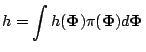 |
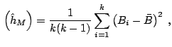
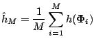
The square root of
![]() is the
numerical standard error of
is the
numerical standard error of
![]() . To describe estimators of
. To describe estimators of
![]() that are consistent in
that are consistent in ![]() , let
, let
![]()
![]() . Then, due to the fact that
. Then, due to the fact that
![]() is a dependent sequence
is a dependent sequence
| Var |
 Cov Cov |
|
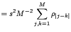 |
||
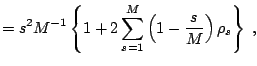 |
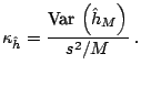
Given the numerical variance it is common to calculate the inefficiency factor, which is also called the autocorrelation time, defined as
 |
(3.9) |

 Cov
Cov