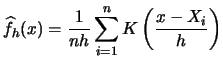
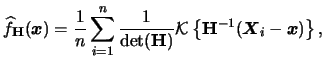
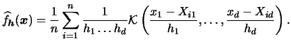
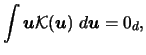
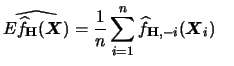
Often one is not only interested in estimating
one-dimensional densities, but also multivariate densities. Recall
e.g. the U.K. Family Expenditure data where we have in fact
observations for
net-income and expenditures on different goods, such as housing, fuel,
food, clothing, durables, transport, alcohol & tobacco etc.
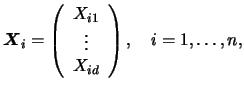
Consider a  -dimensional random vector
 where
where  , ...,
  are one-dimensional random variables.
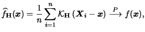
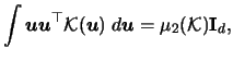
Drawing a random sample of size
are one-dimensional random variables.
Drawing a random sample of size  in this setting means that we
have observations for each of the random variables,
in this setting means that we
have observations for each of the random variables,
 . Suppose that we
collect the
. Suppose that we
collect the  th observation of each of the random variables
in the vector
th observation of each of the random variables
in the vector
 :
:
where  is the th observation of the random variable
  .
Our goal now is to estimate the probability density of
, which is just the joint pdf
.
Our goal now is to estimate the probability density of
, which is just the joint pdf  of the random variables
 |
(3.53) |
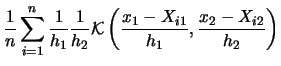
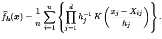
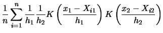
From our previous experience with the one-dimensional case we might
consider adapting the kernel density estimator to the -dimensional
case, and write
 denoting a multivariate kernel function operating
on arguments.
Note, that (3.54) assumes that the bandwidth
denoting a multivariate kernel function operating
on arguments.
Note, that (3.54) assumes that the bandwidth  is the
same for each component. If we relax this assumption then we have a
vector of bandwidths
is the
same for each component. If we relax this assumption then we have a
vector of bandwidths
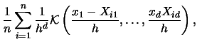
 and the multivariate kernel density estimator becomes
 |
(3.55) |
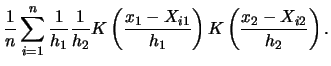
What form should the multidimensional
kernel
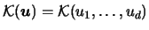 take
on? The easiest solution is to use a multiplicative
kernel
take
on? The easiest solution is to use a multiplicative
kernel
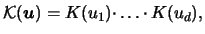 |
(3.56) |
where  denotes a univariate kernel function.
In this case (3.55) becomes
denotes a univariate kernel function.
In this case (3.55) becomes
 |
(3.57) |
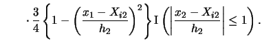
EXAMPLE 3.3
To get a better understanding of what is going on here let us consider
the two-dimensional case where
.
In this case (
3.55) becomes
Each of the
observations is of the form

, where the
first component gives the value that the random variable
takes on at the
th observation and the second component does
the same for

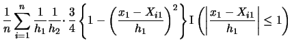
. For illustrational purposes, let us take
to be the Epanechnikov kernel. Then we get
Note that we get a contribution to the sum for observation
only if

falls into the interval
and if

falls into the interval
. If even
one of the two components fails to fall into the respective interval
then one of the indicator functions takes the value 0 and
consequently the observation does not enter the frequency
count.

Note that for kernels with support ![$ [-1,1]$](spmhtmlimg863.gif) (as the Epanechnikov
kernel) observations in a cube around
(as the Epanechnikov
kernel) observations in a cube around
 are used to estimate the
density at the point
.
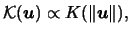
An alternative is to use a true multivariate function
are used to estimate the
density at the point
.
An alternative is to use a true multivariate function
 ,
as e.g. the multivariate Epanechnikov
,
as e.g. the multivariate Epanechnikov
where  denotes proportionality.
These multivariate kernels can be obtained from univariate
kernel functions by taking
denotes proportionality.
These multivariate kernels can be obtained from univariate
kernel functions by taking
 |
(3.59) |
where
 denotes the Euclidean
norm of the vector
denotes the Euclidean
norm of the vector
 .
Kernels of the form (3.59)
use observations from a circle around
to estimate
the pdf at
. This type of kernel is usually called
spherical or radial-symmetric since
has the same value for all
on a sphere around zero.
.
Kernels of the form (3.59)
use observations from a circle around
to estimate
the pdf at
. This type of kernel is usually called
spherical or radial-symmetric since
has the same value for all
on a sphere around zero.
EXAMPLE 3.4
Figure
3.11 shows the contour lines from a bivariate
product and a bivariate radial-symmetric Epanechnikov
kernel, on the left
and right hand side respectively.
Figure:
Contours
from bivariate product (left) and bivariate
radial-symmetric (right) Epanechnikov kernel with equal bandwidths
![\includegraphics[width=0.03\defepswidth]{quantlet.ps}](spmhtmlimg1.gif) SPMkernelcontours
SPMkernelcontours
|
|
Note that the kernel weights in Figure 3.11 correspond
to equal bandwidth in each direction, i.e.
 .
When we use different bandwidths, the observations around
in the density estimate
.
When we use different bandwidths, the observations around
in the density estimate
 will be used
with different weights in both dimensions.
will be used
with different weights in both dimensions.
EXAMPLE 3.5
The contour plots
of product and radial-symmetric Epanechnikov weights with different
bandwidths, i.e.
, are shown
in Figure
3.12. Here we used

and

which
naturally includes fewer observations in the second dimension.
Figure:
Contours from bivariate
product (left) and bivariate radial-symmetric (right)
Epanechnikov kernel with different bandwidths
SPMkernelcontours
|
|
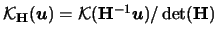
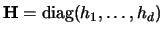
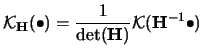
A very general approach is to use a bandwidth matrix
 (nonsingular). The general form for the
multivariate
density estimator is then
(nonsingular). The general form for the
multivariate
density estimator is then
 |
(3.60) |
see Silverman (1986) and Scott (1992).
Here we used the short notation
analogously to  in the one-dimensional case.
A bandwidth matrix includes all simpler cases as special cases.
An equal bandwidth in all dimensions as in (3.54)
corresponds to
in the one-dimensional case.
A bandwidth matrix includes all simpler cases as special cases.
An equal bandwidth in all dimensions as in (3.54)
corresponds to
 where
where
 denotes
the
denotes
the  identity matrix. Different bandwidths as in
(3.55) are equivalent to
identity matrix. Different bandwidths as in
(3.55) are equivalent to
 ,
the diagonal matrix with elements
,
the diagonal matrix with elements
 .
.
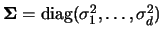
What effect has the inclusion of off-diagonal elements? We will
see in Subsection 3.6.2 that a good rule of thumb is to
use a bandwidth matrix proportional to
 where
where
 is the covariance matrix of the data.
Hence, using such a bandwidth corresponds to a transformation of the
data, so that they have an identity covariance matrix.
As a consequence we can use bandwidth matrices to adjust for
correlation between the components of
is the covariance matrix of the data.
Hence, using such a bandwidth corresponds to a transformation of the
data, so that they have an identity covariance matrix.
As a consequence we can use bandwidth matrices to adjust for
correlation between the components of
 .
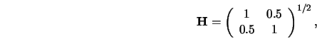
We have plotted the contour curves
of product and radial-symmetric Epanechnikov weights with
bandwidth matrix
.
We have plotted the contour curves
of product and radial-symmetric Epanechnikov weights with
bandwidth matrix
i.e.
 , in Figure 3.13.
Figure:
Contours
from bivariate product (left) and bivariate
radial-symmetric (right) Epanechnikov kernel
with bandwidth matrix
SPMkernelcontours
|
|
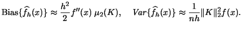
In the following subsection we will consider statistical properties of
bias, variance, the issue
of bandwidth selection and applications for this estimator.
First let us mention that as a consequence of the standard
assumption
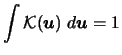 |
(3.61) |
the estimate
 is a density function, i.e.
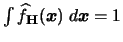 . Also, the
estimate is
consistent in any point
:
. Also, the
estimate is
consistent in any point
:
 |
(3.62) |
see e.g. Ruppert & Wand (1994).
The derivation of  and
and  is principally analogous
to the one-dimensional case. We will only sketch the asymptotic
expansions and hence just move on to the derivation of
is principally analogous
to the one-dimensional case. We will only sketch the asymptotic
expansions and hence just move on to the derivation of  .
.
A detailed derivation of the components of can be
found in Scott (1992) or Wand & Jones (1995)
and the references therein. As in the
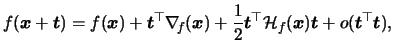
univariate case we use a second order Taylor expansion.
Here and in the following formulae we denote with
 the
gradient
and with
the
gradient
and with
 the Hessian matrix of second partial
derivatives of a function (here ). Then the Taylor
expansion of
the Hessian matrix of second partial
derivatives of a function (here ). Then the Taylor
expansion of
 around
is
around
is
see Wand & Jones (1995, p. 94).
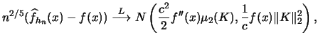
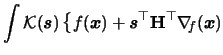
This leads to the expectation
If we assume additionally to (3.61)
| |
|
 |
(3.64) |
| |
|
 |
(3.65) |
then (3.63) yields
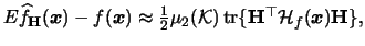 hence
hence
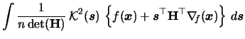
![$\displaystyle \bias\{\widehat{f}_{{\mathbf{H}}}({\boldsymbol{x}})\} \approx\fra...
...mathcal{H}}_{f}({\boldsymbol{x}}){\mathbf{H}}\} \right]^{2}\;d{\boldsymbol{x}}.$](spmhtmlimg906.gif) |
(3.66) |
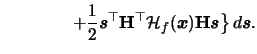
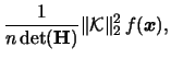
For the variance we find
with
 denoting the -dimensional squared
  -norm
of
.
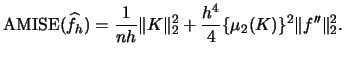
Therefore we have the following formula
for the multivariate kernel density estimator
-norm
of
.
Therefore we have the following formula
for the multivariate kernel density estimator
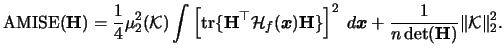 |
(3.68) |
Let us now turn to the problem of how to choose the optimal
bandwidth. Again this is the bandwidth which balances
bias-variance trade-off in .
Denote a scalar, such that
 and
and
 .
Then can be written as
.
Then can be written as
If we only allow changes in the optimal orders for the
smoothing parameter and are
Hence, the multivariate density estimator has a slower rate of
convergence compared to the univariate one, in particular when
is large.
If we consider
 (the same bandwidth in all
dimensions) and we fix the sample size , then
the optimal bandwidth has to be considerably larger than in
the one-dimensional case to make sure that the estimate is reasonably
smooth. Some ideas of comparable sample sizes to reach the same quality
of the density estimates over different dimensions can be
found in Silverman (1986, p. 94) and Scott & Wand (1991).
Moreover, the computational effort of this technique increases with the
number of dimensions . Therefore, multidimensional density
estimation is usually not applied if
(the same bandwidth in all
dimensions) and we fix the sample size , then
the optimal bandwidth has to be considerably larger than in
the one-dimensional case to make sure that the estimate is reasonably
smooth. Some ideas of comparable sample sizes to reach the same quality
of the density estimates over different dimensions can be
found in Silverman (1986, p. 94) and Scott & Wand (1991).
Moreover, the computational effort of this technique increases with the
number of dimensions . Therefore, multidimensional density
estimation is usually not applied if  .
.
The problem of an automatic, data-driven choice of the
bandwidth
has actually more importance for the multivariate than for the
univariate case. In one or two dimensions it is easy to
choose an appropriate bandwidth interactively just by looking at
the plot of density estimates for different bandwidths.
But how can this be done in three, four or more dimensions?
Here arises the problem of graphical representation which we
address in the next subsection.
As in the one-dimensional case,
- plug-in bandwidths, in particular rule-of-thumb bandwidths,
and
- cross-validation bandwidths
are used.
We will introduce generalizations for Silverman's rule-of-thumb
and least squares cross-validation to show the analogy with the
one-dimensional bandwidth selectors.
3.6.2.1 Rule-of-thumb Bandwidth
Rule-of-thumb bandwidth selection gives a formula
arising from the optimal bandwidth for a reference distribution.
Obviously, the pdf of a multivariate normal distribution
 is a good candidate for
a reference distribution
in the multivariate case. Suppose that the kernel
is
multivariate Gaussian, i.e. the pdf of
is a good candidate for
a reference distribution
in the multivariate case. Suppose that the kernel
is
multivariate Gaussian, i.e. the pdf of
 .
Note that
.
Note that
 and
and
 in this case. Hence, from (3.68) and the fact that
cf. Wand & Jones (1995, p. 98),
we can easily derive rule-of-thumb formulae for
different assumptions on
and
 .
.
In the simplest case, i.e. that we consider
and
to be
diagonal matrices
 and
and
 , this
leads to
, this
leads to
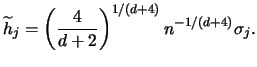 |
(3.69) |
Note that this formula coincides with Silverman's
rule of thumb in
the case  , see (3.24) and
Silverman (1986, p. 45).
Replacing the
, see (3.24) and
Silverman (1986, p. 45).
Replacing the
 s with estimates and noting that the first
factor is always between 0.924 and 1.059, we arrive at Scott's rule:
s with estimates and noting that the first
factor is always between 0.924 and 1.059, we arrive at Scott's rule:
 |
(3.70) |
see Scott (1992, p. 152).
It is not possible to derive the rule-of-thumb for general
and
. However, (3.69) shows that it might be a good idea
to choose the bandwidth matrix
proportional to
 . In
this case we get as a generalization of Scott's rule:
. In
this case we get as a generalization of Scott's rule:
 |
(3.71) |
We remark that this rule is equivalent to applying a Mahalanobis
transformation to the data (to transform the estimated covariance matrix to
identity), then computing the kernel estimate with Scott's
rule (3.70) and finally retransforming
the estimated pdf back to the original scale.
Principally all plug-in methods for the one-dimensional
kernel density estimation can be extended to the multivariate
case. However, in practice this is cumbersome, since the derivation
of asymptotics involves multivariate derivatives
and higher order Taylor expansions.
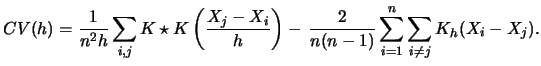
3.6.2.2 Cross-validation
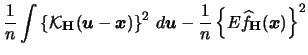
As we mentioned before, the cross-validation method is fairly independent
of the special structure of the parameter or function estimate.
Considering the bandwidth choice problem, cross-validation
techniques allow us to adapt to a wider class of density
functions than the rule-of-thumb approach. (Remember that the
rule-of-thumb bandwidth is optimal for the reference pdf,
hence it will fail for multimodal densities for instance.)
Recall, that in contrast to the rule-of-thumb approach, least squares
cross-validation for density estimation does not estimate
the  optimal but the
  optimal bandwidth.
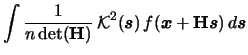
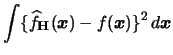
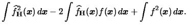
Here we approximate the integrated squared error
optimal bandwidth.
Here we approximate the integrated squared error
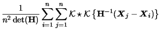
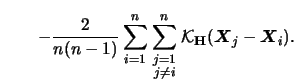
Apparently, this is the same formula as in the one-dimensional case
and with the same arguments the last term of (3.72) can
be ignored. The first term can again be easily calculated
from the data. Hence, only the second term of (3.72) is
unknown and
must be estimated. However, observe that
 , where the only new aspect now
is that
is -dimensional. The resulting expectation, though,
is a scalar.
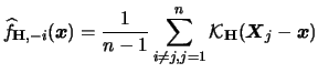
As in (3.32)
we estimate this term by a leave-one-out estimator
where
is simply the multivariate version of (3.33).
Also, the multivariate generalization of (3.37)
is straightforward, which yields the multivariate
cross-validation criterion as a perfect generalization
of
, where the only new aspect now
is that
is -dimensional. The resulting expectation, though,
is a scalar.
As in (3.32)
we estimate this term by a leave-one-out estimator
where
is simply the multivariate version of (3.33).
Also, the multivariate generalization of (3.37)
is straightforward, which yields the multivariate
cross-validation criterion as a perfect generalization
of  in the one-dimensional case:
The difficulty comes in the fact that the bandwidth
is now a matrix
. In the most general
case this means to minimize over  parameters.
Still, if we assume to
a diagonal matrix, this remains
a -dimensional optimization problem.
This holds for other cross-validation approaches, too.
parameters.
Still, if we assume to
a diagonal matrix, this remains
a -dimensional optimization problem.
This holds for other cross-validation approaches, too.
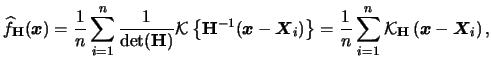
Consider now the problem of graphically displaying
our
multivariate density estimates. Assume first  . Here we are
still able to show the density estimate in a three-dimensional
plot. This is particularly useful if the estimated function can be
rotated interactively on the computer screen. For a two-dimensional
presentation
a contour plot gives often more insight into the structure of the data.
. Here we are
still able to show the density estimate in a three-dimensional
plot. This is particularly useful if the estimated function can be
rotated interactively on the computer screen. For a two-dimensional
presentation
a contour plot gives often more insight into the structure of the data.
Figure:
Two-dimensional density estimate for
age and household income from
East German SOEP 1991
SPMdensity2D
|
|
EXAMPLE 3.6
Figures
3.14 and
3.15
display such a two-dimensional density estimate
for two explanatory variables on East-West German migration intention in
Spring 1991, see Example
1.4. We use the subscript

to indicate
that we used a diagonal bandwidth matrix
.
Aside from some categorical variables on an
educational level, professional status, existence of
relations to
Western Germany and regional dummies, our data set contains
observations on age, household income and environmental
satisfaction.
In Figure
3.14 we plotted the joint density estimate for age
and household income. Additionally Figure
3.15 gives
a contour plot of this density estimate.
It is easily observed that the age distribution
is considerably left skewed.
Figure:
Contour
plot for the two-dimensional density
estimate for age and household income from
East German SOEP 1991
SPMcontour2D
|
|
Here and in the following plots
the bandwidth was chosen according to the general rule of thumb
(3.71), which tends to oversmooth bimodal
structures of the data. The kernel function is always
the product Quartic kernel.
Consider now how to display three- or even higher dimensional
density estimates. One possible approach is to hold one variable
fixed and to plot the
density function only in dependence of the other variables. For
three-dimensional data this
gives three plots:
 vs.
vs.
 ,
,
 vs.
and
vs.
and
 vs.
.
vs.
.
EXAMPLE 3.7
We display this technique
in Figure
3.16 for data from a credit scoring
sample, using duration of the credit, household income and age as
variables (
Fahrmeir & Tutz, 1994).
The title of each panel indicates which variable is held fixed at
which level.
Figure:
Two-dimensional
intersections for the three-dimensional
density estimate for credit duration, household income and age
SPMslices3D
|
|
Figure:
Graphical representation
by contour plot for the three-dimensional
density estimation for credit duration,
household income and age
SPMcontour3D
|
|
EXAMPLE 3.8
Alternatively,
we can plot contours of the density estimate, now in three dimensions,
which means three-dimensional surfaces.
Figure
3.17 shows this for
the credit scoring data.
In the original version of this plot, red, green and blue surfaces
show the values of the density estimate at the levels (in
percent) indicated on the right.
Colors and the possibility of rotating the
contours on the computer screen ease the exploration of the data
structures significantly.
For alternative texts on kernel density estimation we refer to the
monographs by Silverman (1986), Härdle (1990),
Scott (1992) and Wand & Jones (1995).
A particular field of interest and ongoing research is the
matter of bandwidth selection. In addition to what we have
presented, a variety of other cross-validation approaches
and refined plug-in bandwidth selectors have been proposed.
In particular, the following methods are based on the
cross-validation idea:
Pseudo-likelihood
cross-validation
(Duin, 1976; Habbema et al., 1974),
biased cross-validation
(Scott & Terrell, 1987; Cao et al., 1994) and
smoothed cross-validation
(Hall et al., 1992). The latter two approaches also
attempt to find
optimal bandwidths. Hence their performance is also assessed by
relative convergence to the optimal bandwidth  .
A detailed treatment of many cross-validation procedures can be found in
Park & Turlach (1992).
.
A detailed treatment of many cross-validation procedures can be found in
Park & Turlach (1992).
Regarding other refined plug-in bandwidth selectors, the methods
of Sheather and Jones
(Sheather & Jones, 1991) and Hall, Sheather, Jones,
and Marron (Hall et al., 1991) should be mentioned,
as they have have good asymptotic properties ( -convergence).
A number of authors provide
extensive simulation studies for smoothing parameter selection,
we want to mention in particular
Marron (1989),
Jones et al. (1996),
Park & Turlach (1992), and
Cao et al. (1994).
-convergence).
A number of authors provide
extensive simulation studies for smoothing parameter selection,
we want to mention in particular
Marron (1989),
Jones et al. (1996),
Park & Turlach (1992), and
Cao et al. (1994).
A alternative approach is introduced by Chaudhuri & Marron (1999)'s
SiZer (significance zero crossings of derivatives) which tries
to directly find features of a curve, such as bumps and valleys.
At the same time it is a tool for visualizing the estimated
curve at a range of different bandwidth values. SiZer provides
thus a way around the issue of smoothing parameter selection.
EXERCISE 3.1
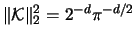
Calculate the exact values of
for the Gaussian, Epanechnikov and Quartic kernels.
EXERCISE 3.3
Show that the density estimate
is itself a pdf if the kernel
is one (i.e. if
).
EXERCISE 3.4
The statistical bureau of Borduria questions

households
about their income. The young econometrician Tintin proposes to use
these data

, ...

for a nonparametric estimate of
the income density

. Tintin suggests computing a confidence
interval for his kernel density estimate
with kernel function
.
Explain how this can be done. Simulate this on the basis of a
lognormal sample with parameters

and

.
EXERCISE 3.8
Derive the formula for

in the case

(Gaussian Kernel).
EXERCISE 3.10
Simulate a mixture of normal densities
with pdf
and plot the density and its estimate with a cross-validated
bandwidth.
EXERCISE 3.13
One possible way to construct a multivariate kernel

is to use a one-dimensional kernel

.
This relationship is given by the formula (
3.59), i.e.
where
.
Find an appropriate constant

for a two-dimensional
a) Gaussian, b) Epanechnikov, and c) Triangle kernel.
EXERCISE 3.14
Show that
. Assume that
possesses a second derivative and

.
EXERCISE 3.15
Explain why averaging over the leave-one-out estimator
(
3.32) is the appropriate way to estimate the
expected value
of

w.r.t. an independent random variable

.
Summary

- Kernel density estimation is a generalization of the
histogram.
The kernel density estimate at point
 corresponds to the histogram bar height for the bin
 if we use the uniform kernel.
- The bias and variance of the kernel density estimator are
- The of the kernel density estimator is
- By using the normal distribution as a reference distribution for
calculating
 we get Silverman's rule-of-thumb bandwidth
which assumes the kernel to be Gaussian.
Other plug-in bandwidths can be found by using more sophisticated
replacements for
.
we get Silverman's rule-of-thumb bandwidth
which assumes the kernel to be Gaussian.
Other plug-in bandwidths can be found by using more sophisticated
replacements for
.
- When using as a goodness-of-fit criterion for
 we can derive the least squares
cross-validation criterion for bandwidth selection:
we can derive the least squares
cross-validation criterion for bandwidth selection:
- The concept of canonical kernels allows us to separate the
kernel choice
from the bandwidth choice. We find a canonical bandwidth
 for each kernel function which gives us the equivalent degree of
smoothing. This equivalence allows one to adjust bandwidths from different
kernel functions to obtain approximately the same value of .
For bandwidth
for each kernel function which gives us the equivalent degree of
smoothing. This equivalence allows one to adjust bandwidths from different
kernel functions to obtain approximately the same value of .
For bandwidth  and kernel
  the bandwidth
is the equivalent bandwidth for kernel
the bandwidth
is the equivalent bandwidth for kernel  .
So for instance, Silverman's rule-of-thumb bandwidth has to be adjusted
by a factor of
.
So for instance, Silverman's rule-of-thumb bandwidth has to be adjusted
by a factor of  for using it with the Quartic kernel.
- The asymptotic normality of the kernel density estimator
allows us to compute confidence intervals for . Confidence bands
can be computed as well, although under more restrictive assumptions on .
- The kernel density estimator for univariate data can be easily
generalized to the multivariate case
where the bandwidth matrix
now replaces the bandwidth
parameter. The multivariate kernel is typically chosen to be
a product or radial-symmetric kernel function. Asymptotic
properties and bandwidth selection are analogous, but more
cumbersome. Canonical bandwidths can be used as well to adjust
between different kernel functions.
A special problem is the graphical display of multivariate density
estimates. Lower dimensional intersections, projections or
contour plot may display only part of the features of a density
function.
![\includegraphics[width=1.4\defpicwidth]{SPMkernelcontoursA.ps}](spmhtmlimg870.gif)
![\includegraphics[width=1.4\defpicwidth]{SPMkernelcontoursB.ps}](spmhtmlimg876.gif)
![\includegraphics[width=1.4\defpicwidth]{SPMkernelcontoursC.ps}](spmhtmlimg890.gif)
![$\displaystyle \amise({\mathbf{H}}) =\frac{1}{4}\,h^{4}\,\mu_{2}^{2}({\mathcal{K...
...ght]^{2}\;d{\boldsymbol{x}}
+ \frac{1}{nh^{d}} \Vert{\mathcal{K}}\Vert^{2}_{2}.$](spmhtmlimg916.gif)
![$\displaystyle {\int [\mathop{\hbox{tr}}\{{\mathbf{H}}^\top{\mathcal{H}}_{f}(x){\mathbf{H}}\}]^{2}\;d{\boldsymbol{x}}}$](spmhtmlimg924.gif)
![$\displaystyle \frac{1}{2^{d+2}{\pi}^{d/2}\mathop{\rm {det}}({\mathbf{\Sigma}})^...
...{\hbox{tr}}({\mathbf{H}}^\top{\mathbf{\Sigma}}^{-1}{\mathbf{H}})\}^{2} \right],$](spmhtmlimg925.gif)
![\includegraphics[width=1.3\defpicwidth]{SPMdensity2D.ps}](spmhtmlimg947.gif)
![\includegraphics[width=1.2\defpicwidth]{SPMcontour2D.ps}](spmhtmlimg951.gif)
![\includegraphics[width=1.4\defpicwidth]{SPMslices3D.ps}](spmhtmlimg956.gif)
![\includegraphics[width=1.3\defpicwidth]{SPMcontour3D.ps}](spmhtmlimg957.gif)