7.2 Estimation Algorithms for PLM and GPLM

In order to estimate the GPLM we consider the same distributional assumptions for $Y$ as in the GLM. Thus we have two cases: (a) the distribution of $Y$ belongs to the exponential family (5.13), or (b) the first two (conditional) moments of $Y$ are specified in order to use the quasi-likelihood function (5.18).

To summarize, the estimation of the GPLM will be based on

$$E(Y\vert{\boldsymbol{U}},{\boldsymbol{T}}) = \mu = G(\eta) = G\{{\boldsymbol{U}}^\top {\boldsymbol{\beta}}+ m({\boldsymbol{T}})\},$$

$$\mathop{\mathit{Var}}(Y\vert{\boldsymbol{U}},{\boldsymbol{T}}) = a(\psi) V(\mu).$$

Recall, that the nuisance parameter $\psi$ is the dispersion parameter (cf. Table 5.2), which is typically given by $a(\psi)=\sigma^2$. In the following we concentrate on the estimation of ${\boldsymbol{\beta}}$ and $m(\bullet)$ since as in the GLM an estimate for the dispersion parameter $\psi$ is easily obtained from (5.25).

The estimation procedures for ${\boldsymbol{\beta}}$ and $m$ can be classified into two categories.

• Profile likelihood type:
  These comprise the profile likelihood and the (generalized) Speckman method. Both methods coincide for the PLM.
• Backfitting type:
  These are based on alternating between parametric and nonparametric estimation. Backfitting was originally developed for AM and GAM. Since the PLM and GPLM can be seen as consisting of two additive components, the backfitting idea applies here as well. We will present backfitting in full detail in Chapters 8 and 9.

7.2.1 Profile Likelihood

The profile likelihood method (considered in Severini & Wong (1992) for this type of problems) is based on the fact, that the conditional distribution of $Y$ given ${\boldsymbol{U}}$ and ${\boldsymbol{T}}$ is parametric. This method starts from keeping ${\boldsymbol{\beta}}$ fixed and to estimate a least favorable (in other words a ``worst case'') nonparametric function $m_{\boldsymbol{\beta}}(\bullet)$ in dependence of the fixed ${\boldsymbol{\beta}}$. The resulting estimate for $m_{\boldsymbol{\beta}}(\bullet)$ is then used to construct the profile likelihood for ${\boldsymbol{\beta}}$. As a consequence the resulting $\widehat{\boldsymbol{\beta}}$ is estimated at $\sqrt{n}$-rate, has an asymptotic normal distribution and is asymptotically efficient (i.e. has asymptotically minimum variance). The nonparametric function $m$ can be estimated consistently by $\widehat{m}(\bullet)=\widehat{m}_{\widehat{{\boldsymbol{\beta}}}}(\bullet)$.

The profile likelihood algorithm can be derived as follows. As explained above we first fix ${\boldsymbol{\beta}}$ and construct the least favorable curve $m_{\boldsymbol{\beta}}$. The parametric (profile) likelihood function is given by

$$\ell({\boldsymbol{Y}},{\boldsymbol{\mu}}_{{\boldsymbol{\beta}}},\... ...ldsymbol{\beta}}+ m_{{\boldsymbol{\beta}}}({\boldsymbol{T}}_{i})\},\psi\right),$$ (7.7)

where ${\boldsymbol{Y}}$ and ${\boldsymbol{\mu}}_{{\boldsymbol{\beta}}}$ denote (in a similar way as in Chapter 5) the corresponding $n$-dimensional vectors for all observations

$${\boldsymbol{Y}}=\left(\begin{array}{c}Y_1\\ \vdots\\ Y_n\end{arr... ...{\beta}}+ m_{{\boldsymbol{\beta}}}({\boldsymbol{T}}_{n})\}\end{array}\right)\,.$$

We maximize (7.7) to obtain an estimate for ${\boldsymbol{\beta}}$. A slightly different objective function is used for the nonparametric part of the model. The smoothed or local likelihood

$$\ell_{{\mathbf{H}}}({\boldsymbol{Y}},{\boldsymbol{\mu}}_{m_{\bold... ...top {\boldsymbol{\beta}}+m_{\boldsymbol{\beta}}({\boldsymbol{t}})\},\psi\right)$$ (7.8)

is maximized to estimate ${m}_{{\boldsymbol{\beta}}}({\boldsymbol{T}})$ at point ${\boldsymbol{T}}$. Here we denote ${\boldsymbol{\mu}}_{m_{\boldsymbol{\beta}}({\boldsymbol{T}})}$ the vector with components $G\{{\boldsymbol{U}}_{i}^\top {\boldsymbol{\beta}}+m_{\boldsymbol{\beta}}({\boldsymbol{T}})\}$. The local weights ${\mathcal{K}}_{{\mathbf{H}}}({\boldsymbol{T}}-{\boldsymbol{T}}_{i})$ are kernel weights with ${\mathcal{K}}$ denoting a (multidimensional) kernel function and ${\mathbf{H}}$ a bandwidth matrix, see Section 3.6.

Denote by $\ell'$, $\ell''$ the first and second derivatives of the $\ell(Y_i,\bullet,\psi)$ w.r.t. its second argument. The maximization of the local likelihood (7.8) at all observations ${\boldsymbol{T}}_j$ requires hence to solve

$$0 = \sum\limits^n_{i=1} {\mathcal{K}}_{{\mathbf{H}}} ({\boldsymbo... ...{\boldsymbol{\beta}}+m_{\boldsymbol{\beta}}({\boldsymbol{t}})\},\psi\right)\, .$$ (7.9)

with respect to $m_{\boldsymbol{\beta}}({\boldsymbol{t}})$. In contrast, the maximization of the profile likelihood (7.7) requires the solution of

$$0 = \sum\limits^n_{i=1} \ell'\left(Y_i,G\{{\boldsymbol{U}}_{i}^\t... ...ol{U}}_i + \gradi_{{\boldsymbol{m}}_{\boldsymbol{\beta}}}({\boldsymbol{T}}_i)\}$$ (7.10)

with respect to the coefficient vector $\beta$. The vector $\gradi_{{\boldsymbol{m}}_{\boldsymbol{\beta}}}$ denotes here the vector of all partial derivatives of $m_{{\boldsymbol{\beta}}}$ with respect to ${\boldsymbol{\beta}}$. A further differentiation of (7.9), this time w.r.t. ${\boldsymbol{\beta}}$, leads to an explicit expression for $\gradi_{{\boldsymbol{m}}_{\boldsymbol{\beta}}}$:

$$\gradi_{{\boldsymbol{m}}_{\boldsymbol{\beta}}}(t)=-\frac{\sum\lim... ... {\boldsymbol{\beta}}+m_{\boldsymbol{\beta}}({\boldsymbol{t}})\}, \psi\right)}.$$ (7.11)

This equation can be used to estimate $\gradi_{{\boldsymbol{m}}_{\boldsymbol{\beta}}}$ in the following derivation of estimators for ${\boldsymbol{\beta}}$ and $m$.

In general, equations (7.9) and (7.10) can only be solved iteratively. Severini & Staniswalis (1994) present a Newton-Raphson type algorithm for this problem. To write the estimation algorithm in a compact form, abbreviate

$$m_j = m_{\boldsymbol{\beta}}({\boldsymbol{T}}_j),$$

$$\ell_i=\ell\left(Y_i,G({\boldsymbol{U}}_{i}^\top {\boldsymbol{\be... ...l\left(Y_i,G({\boldsymbol{U}}_{i}^\top {\boldsymbol{\beta}}+ m_j),\psi\right).$$

Furthermore denote $\ell_i'$, $\ell_i''$, $\ell_{ij}'$, and $\ell_{ij}''$ the first and second derivatives of $\ell_i$ and $\ell_{ij}$ w.r.t. their second argument. Instead of the free parameter ${\boldsymbol{t}}$ we will calculate all values at the observations ${\boldsymbol{T}}_i$. Then, (7.9) and (7.10) transform to

$$= \sum\limits^n_{i=1} \ell'_{ij}\, {\mathcal{K}}_{{\mathbf{H}}} ({\boldsymbol{T}}_i-{\boldsymbol{T}}_j)$$ 0 (7.12)

$$= \sum\limits^n_{i=1} \ell'_i\, \{{\boldsymbol{U}}_i + \gradi_{{\boldsymbol{m}}_i}\}.$$ 0 (7.13)

It is the dependence of $m_i=m_{\boldsymbol{\beta}}({\boldsymbol{T}}_i)$ on ${\boldsymbol{\beta}}$ that adds the additional term $\gradi_{{\boldsymbol{m}}_i}$ (the derivative of $m_i$ w.r.t. ${\boldsymbol{\beta}}$) to the last equation. The estimate of $\gradi_{{\boldsymbol{m}}_i}$ based on (7.11) is therefore necessary to estimate ${\boldsymbol{\beta}}$:

$$\gradi_{{\boldsymbol{m}}_j} = -\,\frac{\sum\limits^n_{i=1} \ell''... ...''_i \, {\mathcal{K}}_{{\mathbf{H}}}({\boldsymbol{T}}_i - {\boldsymbol{T}}_j)}.$$ (7.14)

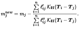
From (7.12) the update step for $m$ (at all observations ${\boldsymbol{T}}_j$) follows directly:

$${m}_j^{new}={m}_j - \frac{\sum\limits_{i=1}^n \ell'_{ij}\, {\math... ...'_{ij}\, {\mathcal{K}}_{{\mathbf{H}}} ({\boldsymbol{T}}_i-{\boldsymbol{T}}_j)}.$$

The Newton-Raphson solution of (7.13) requires a second derivative of $m_{\boldsymbol{\beta}}$. As an approximation consider $\gradi_{{\boldsymbol{m}}_j}$ to be constant with respect to ${\boldsymbol{\beta}}$. This leads to

$${{\boldsymbol{\beta}}}^{new}={{\boldsymbol{\beta}}} - {\mathbf{B}}^{-1} \sum\limits_{i=1}^n \ell'_i\, \widetilde{{\boldsymbol{U}}}_i$$

with a Hessian type matrix

$${\mathbf{B}}=\sum\limits_{i=1}^n \ell''_i\, \widetilde{{\boldsymbol{U}}}_i {\widetilde{{\boldsymbol{U}}}_i^\top }$$

and

$$\widetilde{{\boldsymbol{U}}}_j={\boldsymbol{U}}_j+\gradi_{{\bolds... ...{ij}\, {\mathcal{K}}_{{\mathbf{H}}} ({\boldsymbol{T}}_i-{\boldsymbol{T}}_j)}\,.$$

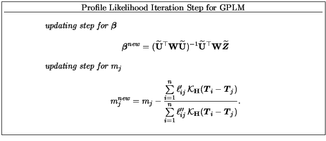
The resulting estimation algorithm consists of iterating the following update steps for ${\boldsymbol{\beta}}$ and $m$ up to convergence. The updating step for $m$ (the nonparametric part) is in general of quite complex structure and cannot be simplified. (Only in some models, in particular for identity and exponential link functions $G$, equation (7.12) can be solved explicitly for $m_j$). It is possible however, to rewrite the updating step for ${\boldsymbol{\beta}}$ in a closed matrix form. Define ${\mathbf{S}}^P$ a smoother matrix with elements

$$({\mathbf{S}}^P)_{ij} = \frac{\ell''_{ij} {\mathcal{K}}_{{\mathbf... ...ell''_{ij}{\mathcal{K}}_{{\mathbf{H}}} ({\boldsymbol{T}}_i-{\boldsymbol{T}}_j)}$$ (7.15)

and let ${\mathbf{U}}$ be the design matrix with rows ${\boldsymbol{U}}_i^\top$. Further denote by ${\mathbf{I}}$ the $n\times n$ identity matrix and

$${\boldsymbol{v}}=(\ell_1',\ldots,\ell_n')^\top\,,\quad {\mathbf{W}}=\mathop{\hbox{diag}}(\ell_1'',\ldots,\ell_n'').$$

Setting $\widetilde{{\mathbf{U}}} = ({\mathbf{I}}-{\mathbf{S}}^P) {\mathbf{U}}$ and $\widetilde{{\boldsymbol{Z}}} = \widetilde{{\mathbf{U}}}{\boldsymbol{\beta}}- {\mathbf{W}}^{-1}{\boldsymbol{v}}$ we can summarize the iteration in the following form:

The variable $\widetilde{{\boldsymbol{Z}}}$ is a sort of adjusted dependent variable. From the formula for ${{\boldsymbol{\beta}}}^{new}$ it becomes clear, that the parameter ${\boldsymbol{\beta}}$ is updated by a parametric method. The only difference to (5.23) is the nonparametric modification of ${{\mathbf{U}}}$ and ${\boldsymbol{Z}}$ resulting in $\widetilde{\mathbf{U}}$ and $\widetilde{\boldsymbol{Z}}$. We remark that as in the GLM case, the functions $\ell''_i$ can be replaced by their expectations (w.r.t. $Y_i$) to obtain a Fisher scoring type procedure.

7.2.2 Generalized Speckman Estimator

The profile likelihood estimator is particularly easy to derive in the case of a PLM, i.e. in particular for the identity link $G$ and normally distributed $Y_i$. Here we have

$$\ell_i'= -(Y_i - {\boldsymbol{U}}_i^\top {\boldsymbol{\beta}}- m_j)/\sigma^2,\quad\textrm{and}\quad \ell_i''\equiv -1/\sigma^2.$$

The latter yields then a simpler smoother matrix ${\mathbf{S}}$ defined by its elements

$$({\mathbf{S}})_{ij} = \frac{ {\mathcal{K}}_{{\mathbf{H}}} ({\bold... ..._{i=1}^n {\mathcal{K}}_{{\mathbf{H}}} ({\boldsymbol{T}}_i-{\boldsymbol{T}}_j)}.$$ (7.16)

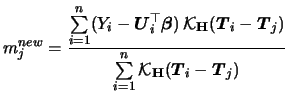
Moreover, the updating step for $m_j$ simplifies to

$${m}_j^{new} = \frac{\sum\limits_{i=1}^n (Y_i - {\boldsymbol{U}}_i... ...s_{i=1}^n {\mathcal{K}}_{{\mathbf{H}}} ({\boldsymbol{T}}_i-{\boldsymbol{T}}_j)}$$

which we can denote in matrix form as

$${{\boldsymbol{m}}}^{new}= {\mathbf{S}}({\boldsymbol{Y}}- {\mathbf{U}}{{\boldsymbol{\beta}}})$$

using again the vector notation for ${\boldsymbol{Y}}$ and similarly for the nonparametric function estimate: ${\boldsymbol{m}}^{new} = \left(m_1^{new},\ldots,m_n^{new}\right)^\top$. For the parameter ${\boldsymbol{\beta}}$ we obtain

$${{\boldsymbol{\beta}}}^{new}=(\widetilde{{\mathbf{U}}}^\top \wide... ...{\mathbf{U}}})^{-1} \widetilde{{\mathbf{U}}}^\top \widetilde{{\boldsymbol{Y}}}$$

using $\widetilde{{\mathbf{U}}} = ({\mathbf{I}}-{\mathbf{S}}) {\mathbf{U}}$ and $\widetilde{{\boldsymbol{Y}}} = ({\mathbf{I}}-{\mathbf{S}}) {\boldsymbol{Y}}$. It turns out that no iteration is necessary. These estimators for the components of a PLM can be summarized as follows:

Now consider the GPLM. We are going to combine the Speckman estimators with the IRLS technique for the GLM (cf. (5.23)). Recall that each iteration step of a GLM was obtained by weighted least squares regression on the adjusted dependent variable. In the same spirit, we estimate the GPLM by replacing the IRLS with a weighted partial linear fit on the adjusted dependent variable. This variable is here given as

$${\boldsymbol{Z}}= {\mathbf{U}}{\boldsymbol{\beta}}+ {\boldsymbol{m}}- {\mathbf{W}}^{-1} {\boldsymbol{v}}.$$ (7.17)

As previously defined, ${\boldsymbol{v}}$ denotes the vector and ${\mathbf{W}}$ denotes the diagonal matrix of the first respectively second derivatives of $\ell_i$.

As for (7.15) we have to introduce weights for the GPLM smoother matrix. The basic simplification in comparison to (7.15) is that we use the matrix ${\mathbf{S}}$ with elements

$$({\mathbf{S}})_{ij} = \frac{\ell''_i {\mathcal{K}}_{{\mathbf{H}}}... ... \ell''_i{\mathcal{K}}_{{\mathbf{H}}} ({\boldsymbol{T}}_i-{\boldsymbol{T}}_j)}.$$ (7.18)

Note the small but important difference in $\ell_i''$ compared to ${\mathbf{S}}^P$. We will come back to the computational simplification in Subsection 7.2.4.

Using the notation $\widetilde{{\mathbf{U}}} = ({\mathbf{I}}-{\mathbf{S}}) {\mathbf{U}}$ and $\widetilde{{\boldsymbol{Z}}} = \widetilde{{\mathbf{U}}}{\boldsymbol{\beta}}- {\mathbf{W}}^{-1}{\boldsymbol{v}}$ (define ${\boldsymbol{v}}$ and ${\mathbf{W}}$ as before), an expression for each iteration step in matrix notation is possible here, too:

There is an important property that this algorithm shares with the backfitting procedure we consider in the next subsection. The updating step for ${\boldsymbol{m}}$ implies

$${\mathbf{S}}{\boldsymbol{Z}}= {\mathbf{S}}{\mathbf{U}}{\boldsymbol{\beta}}+{\boldsymbol{m}}$$

at convergence of the algorithm. Combining this with the definition of ${\boldsymbol{Z}}$ yields

$${\boldsymbol{Z}}-{\mathbf{S}}{\boldsymbol{Z}} = {\mathbf{U}}{\boldsymbol{\beta}}+{\boldsymbol{m}}-{\mathbf{W}}^{-1}{\boldsymbol{v}}-({\mathbf{S}}{\mathbf{U}}{\boldsymbol{\beta}}+{\boldsymbol{m}})$$

$$= ({\mathbf{I}}-{\mathbf{S}}){\mathbf{U}}{\boldsymbol{\beta}}-{\mathbf{W}}^{-1}{\boldsymbol{v}}$$

$$= \widetilde{{\boldsymbol{Z}}}\,.$$

Hence,

$$\widetilde{\boldsymbol{Z}}= ({\mathbf{I}}-{\mathbf{S}}){\boldsymbol{Z}},$$ (7.19)

i.e. $\widetilde{\boldsymbol{Z}}$ is obtained in the same way as $\widetilde{{\mathbf{U}}}$. (Note that we used a different definition when we introduced $\widetilde{{\boldsymbol{Z}}}$.) Equation (7.19) shows that updating the index from ${\mathbf{U}}{\boldsymbol{\beta}}+ {\boldsymbol{m}}$ to ${\mathbf{U}}{\boldsymbol{\beta}}^{new}+{\boldsymbol{m}}^{new}$ is equivalent to determine

$${\mathbf{U}}{\boldsymbol{\beta}}^{new} + {\boldsymbol{m}}^{new} = \MR^S {\boldsymbol{Z}}.$$ (7.20)

Hence, each iteration step corresponds to applying the linear estimation (or hat) matrix $\MR^S$ on the adjusted dependent variable ${\boldsymbol{Z}}$. In order to derive the formula for $\MR^S$, we see from (7.19) that we have at convergence

$${{\mathbf{U}}{\boldsymbol{\beta}}+{\boldsymbol{m}}} = {\mathbf{U}}(\widetilde{{\mathbf{U}}}^\top {\mathbf{W}}\widetilde... ...oldsymbol{Z}}+ {\mathbf{S}}({\boldsymbol{Z}}-{\mathbf{U}}{\boldsymbol{\beta}}),$$ (7.21)

$${{\mathbf{S}}{\mathbf{U}}{\boldsymbol{\beta}}} = {\mathbf{S}}{\mathbf{U}}(\widetilde{{\mathbf{U}}}^\top {\mathbf{W... ...lde{{\mathbf{U}}}^\top {\mathbf{W}}({\mathbf{I}}-{\mathbf{S}}){\boldsymbol{Z}}.$$ (7.22)

Now plugging (7.22) into the right hand side of (7.21) gives

$${{\mathbf{U}}{\boldsymbol{\beta}}+{\boldsymbol{m}}} = \left[\wide... ...mathbf{W}}({\mathbf{I}}- {\mathbf{S}}) + {\mathbf{S}}\right] {\boldsymbol{Z}}.$$

This finally shows that the $\MR^S$ is of the form

$$\MR^S = \widetilde{\mathbf{U}}\{\widetilde{\mathbf{U}}^\top {\mat... ...tilde{\mathbf{U}}^\top {\mathbf{W}}({\mathbf{I}}- {\mathbf{S}}) + {\mathbf{S}}.$$ (7.23)

The linear estimation matrix $\MR^S$ will be used later on to compute approximate degrees of freedom for the semiparametric GPLM estimator.

7.2.3 Backfitting

The backfitting method was originally suggested as an iterative algorithm for fitting an additive model (Buja et al., 1989; Hastie & Tibshirani, 1990). Its key idea is to regress the additive components separately on partial residuals.

Again, let us first consider the PLM

$$E(Y\vert{\boldsymbol{U}},{\boldsymbol{T}}) = {\boldsymbol{U}}^\top {\boldsymbol{\beta}}+ m({\boldsymbol{T}}),$$

which consists of only two additive components. Denote now ${\mathbf{P}}$ the projection matrix

$${\mathbf{P}}= {\mathbf{U}}({\mathbf{U}}^\top {\mathbf{U}})^{-1} {\mathbf{U}}^\top$$

and ${\mathbf{S}}$ a smoother matrix (e.g. the Nadaraya-Watson smoother matrix given by its elements (7.16)). Backfitting means to solve

$${\mathbf{U}}{\boldsymbol{\beta}} = {\mathbf{P}}({\boldsymbol{Y}}- {\boldsymbol{m}})$$

$${\boldsymbol{m}} = {\mathbf{S}}({\boldsymbol{Y}}- {\mathbf{U}}{\boldsymbol{\beta}}).$$

In this case no iteration is necessary and an explicit solution can be given:

$$\widehat{\boldsymbol{\beta}} = \{{\mathbf{U}}^\top ({\mathbf{I}}- {\mathbf{S}}) {\mathbf{U}}\}^{-1} {\mathbf{U}}^\top ({\mathbf{I}}- {\mathbf{S}}) {\boldsymbol{Y}},$$ (7.24)

$$\widehat{\boldsymbol{m}} = {\mathbf{S}}( {\boldsymbol{Y}}-{\mathbf{U}}\widehat{\boldsymbol{\beta}}).$$ (7.25)

We can summarize the estimation procedure in the same way we did for the Speckman estimator. Note the small but subtle difference in the estimate for the parametric part:

We will now extend this technique to the GPLM. The motivation for the backfitting iteration coincides with that for the Speckman iteration. Again we recognize the only difference to Speckman in the updating step for the parametric part. The matrices ${\mathbf{S}}$ and ${\mathbf{W}}$ as well as the vector ${\boldsymbol{v}}$ are defined in exactly the same way as for the Speckman iteration.

It is easy to see that the backfitting algorithm implies a linear estimation matrix for updating the index, too. We have

$${\mathbf{U}}{\boldsymbol{\beta}}^{new} + {\boldsymbol{m}}^{new} = \MR^B {\boldsymbol{Z}}$$

with

$$\MR^B = \widetilde{\mathbf{U}}\{{\mathbf{U}}^\top {\mathbf{W}}\wi... ...{-1} {\mathbf{U}}^\top {\mathbf{W}}({\mathbf{I}}- {\mathbf{S}}) + {\mathbf{S}}.$$ (7.26)

An important caveat of the so defined backfitting procedure is that it may fail with correlated explanatory variables. Hastie & Tibshirani (1990, p. 124ff.) therefore propose a modification of the algorithm (``modified backfitting'', which first searches for a (parametric) solution and only fits the remaining parts nonparametrically. We will introduce this modification later on in Chapter 8.

7.2.4 Computational Issues

Whereas the PLM estimators are directly applicable, all presented algorithms for GPLM are iterative and therefore require an initialization step. Different strategies to initialize the iterative algorithm are possible:

• Start with $\widetilde{{\boldsymbol{\beta}}}$, $\widetilde{m}(\bullet)$ from a parametric (GLM) fit.
• Alternatively, start with ${{\boldsymbol{\beta}}}=0$ and ${m}({\boldsymbol{T}}_j)=G^{-1}(Y_j)$ (for example with the adjustment ${m}_j=G^{-1}\{(Y_j+0.5)/2\}$ for binary responses).
• Backfitting procedures often use ${{\boldsymbol{\beta}}}=0$ and ${m}({\boldsymbol{T}}_j)\equiv G^{-1}(\overline{Y})$.

Next, the smoothing step for the nonparametric function $m(\bullet)$ has to be carried out. Consider the profile likelihood algorithm first. The updating step for $m_j=m_{\boldsymbol{\beta}}({\boldsymbol{T}}_j)$ requires a ratio with numerator and denominator of convolution type

$$\sum_{i=1}^n \delta_{ij} K_{\mathbf{H}}({\boldsymbol{T}}_i-{\boldsymbol{T}}_j),$$ (7.27)

where $\delta_{ij}$ is a derivative of the log-likelihood. Note, that this has to be done at least for all ${\boldsymbol{T}}_j$ ( $j=1,\ldots,n$) since the updated values of $m(\bullet)$ at all observation points are required in the updating step for ${\boldsymbol{\beta}}$. Thus $O(n^2)$ operations are necessary and in each of these operations the kernel function $K_{\mathbf{H}}({\boldsymbol{T}}_i-{\boldsymbol{T}}_j)$ and both likelihood derivatives need to be evaluated.

The essential difference between the profile likelihood and the Speckman algorithm lies in the fact that the former uses $\ell'_i$ and $\ell''_i$ instead of $\ell'_{ij}$ and $\ell''_{ij}$. Thus, both algorithms produce very similar results, when the bandwidth ${\mathbf{H}}$ is small or when $m(\bullet)$ is relatively constant or small with respect to the parametric part. Müller (2001) points out that both estimators very often resemble each other. The comparison of the estimation algorithms can be summarized as follows:

• Backfitting outperforms profile likelihood estimation for a GPLM under independent design. However, if the explanatory variables are dependent, both variants of profile likelihood improve the fit.
• For small sample sizes, the Speckman estimator seems to perform best. The resulting estimator can hence be considered as a good compromise between accuracy and computational efficiency in estimation and specification testing. For larger sample sizes this algorithm gives estimates that are almost identical to the profile likelihood algorithm.

It should be pointed out that this comparison of algorithms is based on Nadaraya-Watson type kernel smoothing. A local linear or local polynomial approach (Fan & Gijbels, 1996) is possible as well. For the particular case of a one-dimensional nonparametric component (i.e. univariate $m$), spline smoothing approaches are often discussed in the literature.

EXAMPLE 7.1  
We consider a subsample of the data used in Examples 5.1 and 5.6. Here we present the estimation results for Mecklenburg-Vorpommern (a state in the very North of Eastern Germany, $n=402$). The data set contains again six explanatory variables, two of them are continuous (age, household income). Descriptive statistics for this subsample are given in Table 7.1.

Table 7.1: Descriptive statistics for migration data (subsample from Mecklenburg-Vorpommern, $n=402$)

		Yes	No	(in %)
$Y$	MIGRATION INTENTION	39.9	60.1
$X_1$	FAMILY/FRIENDS IN WEST	88.8	11.2
$X_2$	UNEMPLOYED/JOB LOSS CERTAIN	21.1	78.9
$X_3$	CITY SIZE 10,000-100,000	35.8	64.2
$X_4$	FEMALE	50.2	49.8
		Min	Max	Mean	S.D.
$X_5$	AGE (in years)	18	65	39.93	12.89
$T$	HOUSEHOLD INCOME (in DM)	400	4000	2262.22	769.82

For illustration purposes we restrict ourselves to considering only one continuous variable (household income) for the nonparametric part. Table 7.2 shows on the left the coefficients of the parametric logit fit. The estimated coefficients for the parametric part of the GPLM are given on the right side of Table 7.2. For easier assessment of the coefficients, both continuous variables (age, household income) have been linearly transformed to $[0,1]$. We see that the migration intention is definitely determined by age ($X_5$). However, the coefficients of unemployment ($X_2$), city size ($X_3$) and household income ($T$) variables are also highly significant.

Table 7.2: Logit and GPLM coefficients for migration data, $h=0.3$

					Modified
	Logit ($t$ value)	Profile	Speckman	Backfitting	Backfitting
const.	-0.358 (-0.68)	--	--	--	--
$X_1$	0.589 ( 1.54)	0.600 ( 1.56)	0.599 ( 1.56)	0.395	0.595
$X_2$	0.780 ( 2.81)	0.800 ( 2.87)	0.794 ( 2.85)	0.765	0.779
$X_3$	0.822 ( 3.39)	0.842 ( 3.47)	0.836 ( 3.45)	0.784	0.815
$X_4$	-0.388 (-1.68)	-0.402 (-1.73)	-0.400 (-1.72)	-0.438	-0.394
$X_5$	-3.364 (-6.92)	-3.329 (-6.86)	-3.313 (-6.84)	-3.468	-3.334
$T$	1.084 ( 1.90)	--	--	--	--
	Linear (GLM)	Part. Linear (GPLM)

Figure: GPLM logit fit for migration data, generalized Speckman estimator for $m$ using $h=0.3$ (thick curve), $h=0.2$, $h=0.25$, $h=0.35$, $h=0.4$ (thin curves) and parametric logit fit (straight line)
SPMmigmv

The nonparametric estimate $\widehat{m}(\bullet)$ in this example seems to be an obvious nonlinear function, see Figure 7.1. As already observed in the simulations, both profile likelihood methods give very similar results. Also the nonparametric curves from backfitting and modified backfitting do not differ much from those of the profile likelihood approaches. The reason is the very similar smoothing step in all four methods. We show therefore only a plot of the curves obtained from the generalized Speckman algorithm.

Table 7.2 shows on the right hand side the parameter estimates for all semiparametric estimates. For the generalized Speckman method, the matrix $a(\widehat{\psi})(\widetilde{{\mathbf{U}}}^\top {\mathbf{W}}\widetilde{{\mathbf{U}}})^{-1}$ with $\widetilde{{\mathbf{U}}}$ and ${\mathbf{W}}$ from the last iteration can be used as an estimate for the covariance matrix of $\widehat{\boldsymbol{\beta}}$. We present the calculated $t$-values from this matrix. Note that $a(\psi)=1$ for binary $Y$, so we omit this factor here. An analogous approach is possible for the profile likelihood method, see Severini & Staniswalis (1994). Here we can estimate the covariance of $\widehat{\boldsymbol{\beta}}$ by $a(\widehat{\psi})(\widetilde{{\mathbf{U}}}^\top {\mathbf{W}}\widetilde{{\mathbf{U}}})^{-1}$, now using the appropriate smoother matrix ${\mathbf{S}}^P$ instead of ${{\mathbf{S}}}$.

The obvious difference between backfitting and the other procedures in the estimated effect of $X_1$ is an interesting observation. It is most likely due to the multivariate dependence structure within the explanatory variables, an effect which is not easily reflected in simulations. The profile likelihood methods have by construction a similar correction ability for concurvity as the modified backfitting has. $\Box$