Next: 9.4 Linear Regression
Up: 9. Robust Statistics
Previous: 9.2 Location and Scale
Subsections
9.3 Location and Scale in

9.3.1 Equivariance and Metrics
In Sect. 9.2.1 we discussed the equivariance of estimators
for location and scale with respect to the affine group of transformations on
 . This
carries over to higher dimensions although here the requirement of
affine equivariance lacks immediate
plausibility. A change of location and scale for each individual component in
. This
carries over to higher dimensions although here the requirement of
affine equivariance lacks immediate
plausibility. A change of location and scale for each individual component in
 is represented by an affine transformation of the form
 where
where  is a diagonal matrix. A general affine
transformation forms linear combinations of the individual components which
goes beyond arguments based on units of measurement. The use of affine
equivariance reduces to the almost empirical question as to whether the data,
regarded as a cloud of points in
, can be well represented by an
ellipsoid. If this is the case as it often is then consideration of linear
combinations of different components makes data analytical sense. With this
proviso in mind we consider the affine group
is a diagonal matrix. A general affine
transformation forms linear combinations of the individual components which
goes beyond arguments based on units of measurement. The use of affine
equivariance reduces to the almost empirical question as to whether the data,
regarded as a cloud of points in
, can be well represented by an
ellipsoid. If this is the case as it often is then consideration of linear
combinations of different components makes data analytical sense. With this
proviso in mind we consider the affine group
 of
transformations of
into itself,
of
transformations of
into itself,
 |
(9.67) |
where  is a non-singular
  -matrix and
  is an
arbitrary point in
. Let
is an
arbitrary point in
. Let
 denote a family of
distributions over
which is closed under affine
transformations
denote a family of
distributions over
which is closed under affine
transformations
 for all for all  |
(9.68) |
A function
 is called a location functional if it
is well defined and
is called a location functional if it
is well defined and
 for all for all  |
(9.69) |
A functional
 where
where
 denotes the set of all strictly positive definite
symmetric
matrices is called a scale or scatter functional if
denotes the set of all strictly positive definite
symmetric
matrices is called a scale or scatter functional if
The requirement of affine equivariance is a strong one as we now
indicate. The most obvious way of defining the median of a
 -dimensional data set is to define it by the medians of the
individual components. With this definition the median
is equivariant with respect to transformations of the form
with a diagonal matrix but it is not
equivariant for the affine group. A second possibility is to define
the median of a distribution
-dimensional data set is to define it by the medians of the
individual components. With this definition the median
is equivariant with respect to transformations of the form
with a diagonal matrix but it is not
equivariant for the affine group. A second possibility is to define
the median of a distribution  by
by
With this definition the median is equivariant with respect to
transformations of the form
 with
with  an
orthogonal matrix but not with respect to the affine group or the
group
an
orthogonal matrix but not with respect to the affine group or the
group
 with a diagonal
matrix. The conclusion is that there is no canonical extension of the
median to higher dimensions which is equivariant with respect to the
affine group.
with a diagonal
matrix. The conclusion is that there is no canonical extension of the
median to higher dimensions which is equivariant with respect to the
affine group.
In Sect. 9.2 use was made of metrics on the space of
probability distributions on
. We extend this to
where all metrics we consider are of the form
 |
(9.71) |
where
 is a so called
Vapnik-Cervonenkis class (see for example Pollard (1984)).
The class
can be chosen to suit
the problem. Examples are the class of all lower dimensional
hyperplanes
is a so called
Vapnik-Cervonenkis class (see for example Pollard (1984)).
The class
can be chosen to suit
the problem. Examples are the class of all lower dimensional
hyperplanes
These give rise to the metrics
 and
and
 respectively. Just as in
metrics
respectively. Just as in
metrics
 of the form
(9.71) allow direct comparisons between empirical measures and
models. We have
of the form
(9.71) allow direct comparisons between empirical measures and
models. We have
 |
(9.74) |
uniformly in (see [80]).
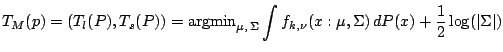
9.3.2 M-estimators of Location and Scale
Given the usefulness of M-estimators for one
dimensional data it seems
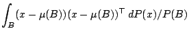
natural to extend the concept to higher dimensions. We follow [68]. For any positive definite symmetric -matrix
 we define the metric
 by
by
Further, let  and
and  be two non-negative continuous functions
defined on
be two non-negative continuous functions
defined on
 and be such that
 are both
bounded. For a given probability distribution on the Borel sets of
we consider in analogy to (9.21) and (9.22) the two
equations in
are both
bounded. For a given probability distribution on the Borel sets of
we consider in analogy to (9.21) and (9.22) the two
equations in  and
and
Assuming that at least one solution
 exists we denote it
by
exists we denote it
by
 . The existence of a solution of (9.75)
and (9.76) can be shown under weak conditions as
follows. If we define
. The existence of a solution of (9.75)
and (9.76) can be shown under weak conditions as
follows. If we define
 |
(9.77) |
with
 as in (9.73) then a solution exists if
 where
where  depends only on the functions
and ([68]). Unfortunately the problem of
uniqueness is much more difficult than in the one-dimensional
case. The conditions placed on in [68] are either that it has a density
depends only on the functions
and ([68]). Unfortunately the problem of
uniqueness is much more difficult than in the one-dimensional
case. The conditions placed on in [68] are either that it has a density  which is
a decreasing function of
which is
a decreasing function of
 or that it is symmetric
 for every Borel set
  . Such conditions do not hold
for real data sets which puts us in an awkward position.
Furthermore without existence and uniqueness there can be no
results on asymptotic normality and
consequently no results on confidence
intervals. The situation is unsatisfactory so we now turn to the
one class of M-functionals for which
existence and uniqueness can be shown. The following is
based on [61] and is the multidimensional generalization of
(9.33). The -dimensional
. Such conditions do not hold
for real data sets which puts us in an awkward position.
Furthermore without existence and uniqueness there can be no
results on asymptotic normality and
consequently no results on confidence
intervals. The situation is unsatisfactory so we now turn to the
one class of M-functionals for which
existence and uniqueness can be shown. The following is
based on [61] and is the multidimensional generalization of
(9.33). The -dimensional  -distribution with density
 is defined by
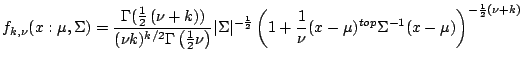 |
(9.78) |
and we consider the minimization problem
 |
(9.79) |
where
 denotes the determinant of the positive
definite matrix . For any distribution on the Borel
sets of
we define
denotes the determinant of the positive
definite matrix . For any distribution on the Borel
sets of
we define
 which is the
-dimensional version of (9.23). It can be shown that if
which is the
-dimensional version of (9.23). It can be shown that if
 then (9.79) has a unique solution.
Moreover for data sets there is a simple algorithm which
converges to the solution. On differentiating the right hand side
of (9.79) it is seen that the solution is an
M-estimator as in (9.75) and
(9.76). Although this has not been proven explicitly it
seems clear that the solution will be locally uniformly
Fréchet differentiable,
that is, it will satisfy (9.12) where the influence
function
then (9.79) has a unique solution.
Moreover for data sets there is a simple algorithm which
converges to the solution. On differentiating the right hand side
of (9.79) it is seen that the solution is an
M-estimator as in (9.75) and
(9.76). Although this has not been proven explicitly it
seems clear that the solution will be locally uniformly
Fréchet differentiable,
that is, it will satisfy (9.12) where the influence
function
 can be obtained as in (9.54) and the
metric
can be obtained as in (9.54) and the
metric  is replaced by the metric
 . This
together with (9.74) leads to uniform asymptotic
normality and allows the construction of confidence regions. The
only weakness of the proposal is the low gross error
breakdown point
. This
together with (9.74) leads to uniform asymptotic
normality and allows the construction of confidence regions. The
only weakness of the proposal is the low gross error
breakdown point
 defined below which is at most
  . This upper bound is
shared with the M-functionals defined
by (9.75) and (9.76) ([68]). The problem of
constructing high breakdown functionals in dimensions will be
discussed below.
. This upper bound is
shared with the M-functionals defined
by (9.75) and (9.76) ([68]). The problem of
constructing high breakdown functionals in dimensions will be
discussed below.
9.3.3 Bias and Breakdown
The concepts of bias and breakdown developed in Sect. 9.2.4 carry over to
higher dimensions. Given a metric  on the space of distributions on
and a location functional
on the space of distributions on
and a location functional  we
follow (9.37) and define
we
follow (9.37) and define
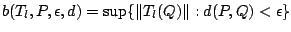 |
(9.80) |
and
 |
(9.81) |
where by convention
 if is not defined at
 . The extension to scale functionals is not so obvious
as there is no canonical definition of bias. We require
a measure of difference between two positive definite symmetric
matrices. For reasons
of simplicity and because it is sufficient for
our purposes the one we take is
. The extension to scale functionals is not so obvious
as there is no canonical definition of bias. We require
a measure of difference between two positive definite symmetric
matrices. For reasons
of simplicity and because it is sufficient for
our purposes the one we take is
 .
Corresponding to (9.36) we define
.
Corresponding to (9.36) we define
 |
(9.82) |
and
 |
(9.83) |
Most work is done using the gross error model
(9.81) and
(9.83).
The breakdown points of are defined by
where (9.86) corresponds in the obvious manner to
(9.41). The breakdown points for the scale functional  are defined analogously using the bias
functional (9.82). We have
are defined analogously using the bias
functional (9.82). We have
Theorem 4
For any translation equivariant functional
 and and  |
(9.87) |
and for any affine equivariant scale functional
 and and  |
(9.88) |
In Sect. 9.2.4 it was shown that the M-estimators of
Sect. 9.2.3 can attain or almost attain the upper bounds
of Theorem 1. Unfortunately this is not the case in
dimensions where as we have already mentioned the breakdown points of M-functionals of
Sect. 9.3.2 are at most . In recent years much
research activity has been directed towards finding high breakdown
affinely equivariant location and scale functionals which attain
or nearly attain the upper bounds of Theorem 4. This is
discussed in the next section.
The first high breakdown affine
equivariant location and scale functionals were proposed independently of each other by
[103] and [31].
They were defined for empirical data but the
construction can be carried over to measures satisfying a certain
weak condition. The idea is to project the data points onto lines
through the origin and then to determine which points are outliers
with respect to this projection using one-dimensional functions with
a high breakdown point. More precisely we set
 |
(9.89) |
and
 |
(9.90) |
This is a measure for the outlyingness of the point  and it may be
checked that it is affine invariant. Location and scale functionals may now be
obtained by taking for example the mean and the covariance matrix of those
and it may be
checked that it is affine invariant. Location and scale functionals may now be
obtained by taking for example the mean and the covariance matrix of those
 observations with the smallest outlyingness measure.
Although (9.90) requires a supremum over all values of
observations with the smallest outlyingness measure.
Although (9.90) requires a supremum over all values of  this
can be reduced for empirical distributions as follows. Choose all linearly
independent subsets
this
can be reduced for empirical distributions as follows. Choose all linearly
independent subsets
 of size and for each such
subset determine a which is orthogonal to their span. If the
of size and for each such
subset determine a which is orthogonal to their span. If the  in (9.90) is replaced by a maximum over all such then the
location and scale functionals remain affine equivariant and retain the high
breakdown point. Although this requires the consideration of only a finite
number of directions namely at most
in (9.90) is replaced by a maximum over all such then the
location and scale functionals remain affine equivariant and retain the high
breakdown point. Although this requires the consideration of only a finite
number of directions namely at most
 this number is too large to make it a practicable
possibility even for small values of
this number is too large to make it a practicable
possibility even for small values of  and . The problem of calculability
has remained with high breakdown methods ever since and it is their main
weakness. There are still no high breakdown affine equivariant functionals
which can be calculated exactly except for very small
data sets. [60] goes as far as to say that the problem of
calculability is the breakdown of high breakdown methods. This is
perhaps too
pessimistic but the problem remains unsolved.
and . The problem of calculability
has remained with high breakdown methods ever since and it is their main
weakness. There are still no high breakdown affine equivariant functionals
which can be calculated exactly except for very small
data sets. [60] goes as far as to say that the problem of
calculability is the breakdown of high breakdown methods. This is
perhaps too
pessimistic but the problem remains unsolved.
[89] introduced two further high breakdown location and scale functionals as follows. The first, the so
called minimum volume ellipsoid (MVE) functional, is a multidimensional
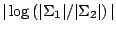
version of Tukey's shortest half-sample (9.8) and is defined as follows. We set
 |
(9.91) |
where
 denotes the volume of
  and
and
 denotes the number of elements of the set
  . In other words
has the smallest volume of any ellipsoid which contains more than
half the data points. For a general distribution we define
. In other words
has the smallest volume of any ellipsoid which contains more than
half the data points. For a general distribution we define
 |
(9.92) |
Given the location functional  is defined to be the centre
  of
and the covariance functional
of
and the covariance functional  is taken to be
 where
where
 |
(9.93) |
The factor  can be chosen so that
 for
the standard normal distribution in dimensions.
for
the standard normal distribution in dimensions.
The second functional is based on the so called minimum covariance
determinant (MCD) and is as follows. We write
and define
 |
(9.96) |
where
 is
defined to be infinite if either of (9.94) or (9.95) does
not exist. The location functional is taken to be
is
defined to be infinite if either of (9.94) or (9.95) does
not exist. The location functional is taken to be
 and the scatter functional
 where again
is usually chosen so that
where again
is usually chosen so that
 for
the standard normal distribution in -dimensions. It can be shown
that both these functionals are affinely equivariant.
for
the standard normal distribution in -dimensions. It can be shown
that both these functionals are affinely equivariant.
A smoothed version of the minimum volume estimator can be obtained by
considering the minimization problem
minimize  subject to subject to  |
(9.97) |
where
![$ \rho: \mathbb{R}_{+} \rightarrow [0,\,1]$](img5729.gif) satisfies
satisfies
 and is continuous on the right
(see [23]). This gives rise to the class of so called
and is continuous on the right
(see [23]). This gives rise to the class of so called
 -functionals. The minimum volume estimator
can be obtained by
specializing to the case
-functionals. The minimum volume estimator
can be obtained by
specializing to the case
 .
.
On differentiating (9.97) it can be seen that an -functional
can be regarded as an M-functional but with redescending functions
and in contrast to the conditions placed on and
in (9.75) and (9.76) ([64]). For such functions the defining equations for an
M-estimator have many solutions and the minimization problem of
(9.97) can be viewed as a choice function. Other choice
functions can be made giving rise to different high breakdown
M-estimators. We refer to
[65] and [62].
A further class of
location and scatter functionals have been developed from Tukey's
concept of depth ([109]). We refer to
[32], [63] and Zuo and Serfling (2000a, 2000b).
Many of the above functionals have breakdown points
close to or equal to the upper bound of Theorem 4. For the
calculation of breakdown points we refer to
Davies (1987, 1993), [66], [32] and [111].
The problem of determining a functional which minimizes the
bias over a neighbourhood was considered in the
one-dimensional case in Sect. 9.2.4. The problem is much more
difficult in
but some
work in this direction has been done (see [1]). The more tractable problem of determining
the size of the bias function for particular
functionals or classes of functionals has also been
considered ([115,69]).
All the above functionals can be shown to exist but there are problems
concerning the uniqueness of the functional. Just as in the case of
Tukey's shortest half (9.8) restrictions must be placed on
the distribution which generally include the existence of
a density with given properties
(see [23] and [105]) and which is
therefore at odds with the spirit of robust statistics. Moreover even
uniqueness and asymptotic normality at some small class of models are not sufficient. Ideally the functional should
exist and be uniquely defined and locally uniformly Fréchet differentiable just as
in Sect. 9.2.5. It is not easy to construct affinely equivariant location and scatter functionals
which satisfy the first two conditions but it has been
accomplished by [30] using the Stahel-Donoho idea of
projections described above. To go further and define functionals
which are also locally uniformly Fréchet differentiable with
respect to some metric
 just as in the one-dimensional
case considered in Sect. 9.2.5 is a very difficult
problem. The only result in this direction is again due to [30] who managed to construct functionals which are locally
uniformly Lipschitz. The lack of locally uniform Fréchet
differentiability means that all derived confidence intervals will
exhibit a certain degree of instability. Moreover the problem is
compounded by the inability to calculate the functionals
themselves. To some extent it is possible to reduce the instability by
say using the MCD functional in preference to the MVE functional, by
reweighting the observations or by calculating a one-step M-functional
as in (9.29)
(see [24]).
However the problem
remains and for this reason we do not discuss the research which has
been carried out on the efficiency of the location and scatter
functionals mentioned above. Their main use is in data analysis where
they are an invaluable tool for detecting
outliers. This will be discussed in the following section.
just as in the one-dimensional
case considered in Sect. 9.2.5 is a very difficult
problem. The only result in this direction is again due to [30] who managed to construct functionals which are locally
uniformly Lipschitz. The lack of locally uniform Fréchet
differentiability means that all derived confidence intervals will
exhibit a certain degree of instability. Moreover the problem is
compounded by the inability to calculate the functionals
themselves. To some extent it is possible to reduce the instability by
say using the MCD functional in preference to the MVE functional, by
reweighting the observations or by calculating a one-step M-functional
as in (9.29)
(see [24]).
However the problem
remains and for this reason we do not discuss the research which has
been carried out on the efficiency of the location and scatter
functionals mentioned above. Their main use is in data analysis where
they are an invaluable tool for detecting
outliers. This will be discussed in the following section.
A scatter matrix plays an important role in many statistical
techniques such as principal component analysis and factor
analysis. The use of robust
scatter functionals in some of these areas has been studied by
among others
[21], [20] and [113].
As already mentioned the major weakness of all known high breakdown functionals is their
computational complexity. For the MCD functional an exact algorithm of
the order of
 exists and there are reasons for supposing
that this cannot be reduced to below
exists and there are reasons for supposing
that this cannot be reduced to below  ([12]).
This means that in practice for all but very
small data sets heuristic algorithms have to be used. We refer to
[95] for a heuristic algorithm for the MCD-functional.
([12]).
This means that in practice for all but very
small data sets heuristic algorithms have to be used. We refer to
[95] for a heuristic algorithm for the MCD-functional.
Whereas for univariate, bivariate and even trivariate data
outliers may often be found by visual inspection,
this is not practical in higher dimensions
([16,49,4,48,50]).
This makes it all the more important to
have methods which automatically detect high dimensional
outliers. Much of the analysis of the one-dimensional problem given in
Sect. 9.2.7 carries over to the -dimensional
problem. In particular outlier identification rules based on the mean
and covariance of the data suffer from masking problems and must be
replaced by high breakdown functionals
(see also Rocke and Woodruff (1996, 1997)). We restrict attention to
affine equivariant functionals so that
an affine transformation of the data will not alter the
observations which are identified as outliers. The identification
rules we consider are of the form
 |
(9.98) |
where  is the empirical measure, and are affine
equivariant location and scatter functionals respectively and
is the empirical measure, and are affine
equivariant location and scatter functionals respectively and  is a constant to be determined. This rule is the -dimensional
counterpart of (9.60). In order to specify some reasonable
value for and in order to be able to compare different
outlier identifiers we require, just as in Sect. 9.2.7,
a precise definition of an outlier and a basic model for the majority
of the observations. As our basic model we take the -dimensional
normal distribution
is a constant to be determined. This rule is the -dimensional
counterpart of (9.60). In order to specify some reasonable
value for and in order to be able to compare different
outlier identifiers we require, just as in Sect. 9.2.7,
a precise definition of an outlier and a basic model for the majority
of the observations. As our basic model we take the -dimensional
normal distribution
 . The definition of an
 -outlier corresponds to (9.62) and is
 |
(9.99) |
where
 for some given value of
 .
Clearly for an i.i.d. sample of size distributed
according to
the probability that no
observation lies in the outlier region of (9.99) is just
.
Clearly for an i.i.d. sample of size distributed
according to
the probability that no
observation lies in the outlier region of (9.99) is just
 . Given location and scale functionals and and
a sample
. Given location and scale functionals and and
a sample
 we write
 |
(9.100) |
which corresponds to (9.64). The region
 is the empirical counterpart of
 of (9.99) and any
observation lying in
will be
identified as an outlier. Just as in the one-dimensional case we
determine the
of (9.99) and any
observation lying in
will be
identified as an outlier. Just as in the one-dimensional case we
determine the
 by requiring that with probability
 no observation is identified as an outlier in
i.i.d.
samples of size . This can be
done by simulations with appropriate asymptotic approximations for
large . The simulations will of course be based on the
algorithms used to calculate the functionals and will not be based
on the exact functionals assuming these to be well defined. For
the purpose of outlier
identification this will not be of great consequence. We give
results for three multivariate outlier identifiers based on the
MVE- and
MCD-functionals of [89] and the -functional based on
Tukey's biweight function as given in [84]. There are good
heuristic algorithms for calculating these functionals at least
approximately
([84,95,97]).
The following is based on [8].
Table 9.2 gives the values of
with
no observation is identified as an outlier in
i.i.d.
samples of size . This can be
done by simulations with appropriate asymptotic approximations for
large . The simulations will of course be based on the
algorithms used to calculate the functionals and will not be based
on the exact functionals assuming these to be well defined. For
the purpose of outlier
identification this will not be of great consequence. We give
results for three multivariate outlier identifiers based on the
MVE- and
MCD-functionals of [89] and the -functional based on
Tukey's biweight function as given in [84]. There are good
heuristic algorithms for calculating these functionals at least
approximately
([84,95,97]).
The following is based on [8].
Table 9.2 gives the values of
with
 . The results are based on
  simulations for each combination of and .
[8] show by simulations that although none of the
above rules fails to detect arbitrarily large outliers it still can
happen that very extreme observations are not identified as outliers. To
quantify this we consider the identifier
 and the
constellation
and the
constellation  with
with  observations replaced by other values.
The mean norm of the most extreme nonidentifiable outlier is 4.17. The
situation clearly becomes worse with an increasing proportion of
replaced observations and with the dimension
(see [7]).
If we use the mean of the norm of the most extreme
non-identifiable outlier as a criterion then none of the three rules
dominates the others although the biweight identifier performs
reasonably well in all cases and is our preferred choice.
observations replaced by other values.
The mean norm of the most extreme nonidentifiable outlier is 4.17. The
situation clearly becomes worse with an increasing proportion of
replaced observations and with the dimension
(see [7]).
If we use the mean of the norm of the most extreme
non-identifiable outlier as a criterion then none of the three rules
dominates the others although the biweight identifier performs
reasonably well in all cases and is our preferred choice.
Table 9.2:
Normalizing constants
for OR ,
OR
,
OR , OR
, OR for
for
|
|
 |
 |
 |
 |
 |
 |
 |
 |
|
 |
 |
 |
 |
|
 |
 |
 |
 |
 |
|
 |
 |
 |
|
|
 |
 |
 |
|
|
 |
 |
 |
Next: 9.4 Linear Regression
Up: 9. Robust Statistics
Previous: 9.2 Location and Scale